Advanced text functions in Google Sheets

In this tutorial, you will be introduced to four advanced text functions in Google Sheets. Often, you have data that is not in the desired format, so you need to edit and adjust it. With the help of these functions, you will be able to transform your text data and make it usable for your specific needs.

Key Takeaways

You will learn how to use the UPPER and LOWER functions to convert text to uppercase or lowercase, how to replace characters in your text data using the SUBSTITUTE function, how to remove excess spaces with the TRIM function, and how the REPLACE function works to replace specific words in a text.

Step-by-step Guide

Step 1: Using the UPPER Function

First, let's look at the UPPER function, which allows you to convert a string to uppercase. You have a list of states in Germany that you want to convert to uppercase. Enter the following formula into cell F3:

=UPPER(B3)

Here is the screenshot showing you how the function is applied:

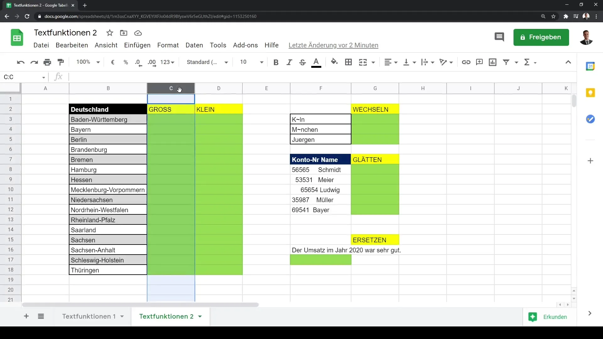
Since you can drag this formula down, you will automatically get the other entries in the list.

Step 2: Using the LOWER Function

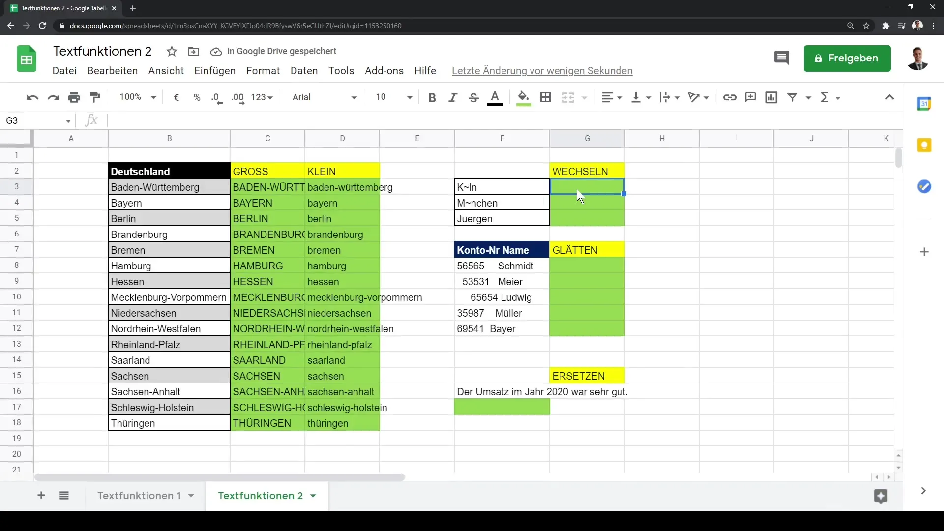
Now, let's achieve the opposite and present the same data in lowercase. To do this, use the LOWER function, which you enter in cell F6 as follows:

=LOWER(B3)

As a result, you have the option to drag this formula down as well to convert all further data to lowercase.

Step 3: Using the SUBSTITUTE Function

Now let's move on to the SUBSTITUTE function. This function allows you to replace a specific character in a text with another character. This is particularly useful if you want to switch from one special character to another. To use the function, go to cell F10 and enter the following:

=SUBSTITUTE(B3; "ö"; "Ö")

Here you can place the character you want to replace in quotes and add your desired new character. This screenshot shows you the application of the SUBSTITUTE function:

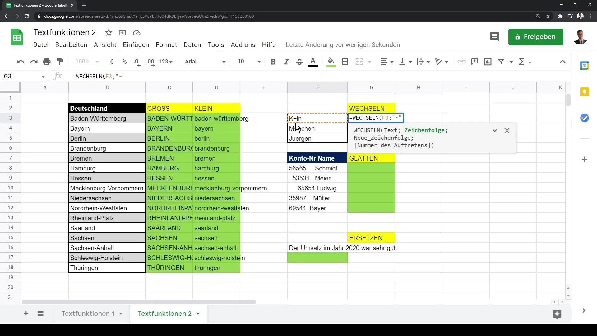
Make sure to replace the appropriate character for each specific case.

Step 4: Using the TRIM Function

Next, let's look at the TRIM function, which is used to remove spaces in a text. Simply enter the following formula in cell F12:

=TRIM(B3)

After entering the formula, drag it down so that the spaces in all subsequent cells are removed.

Step 5: Using the REPLACE Function

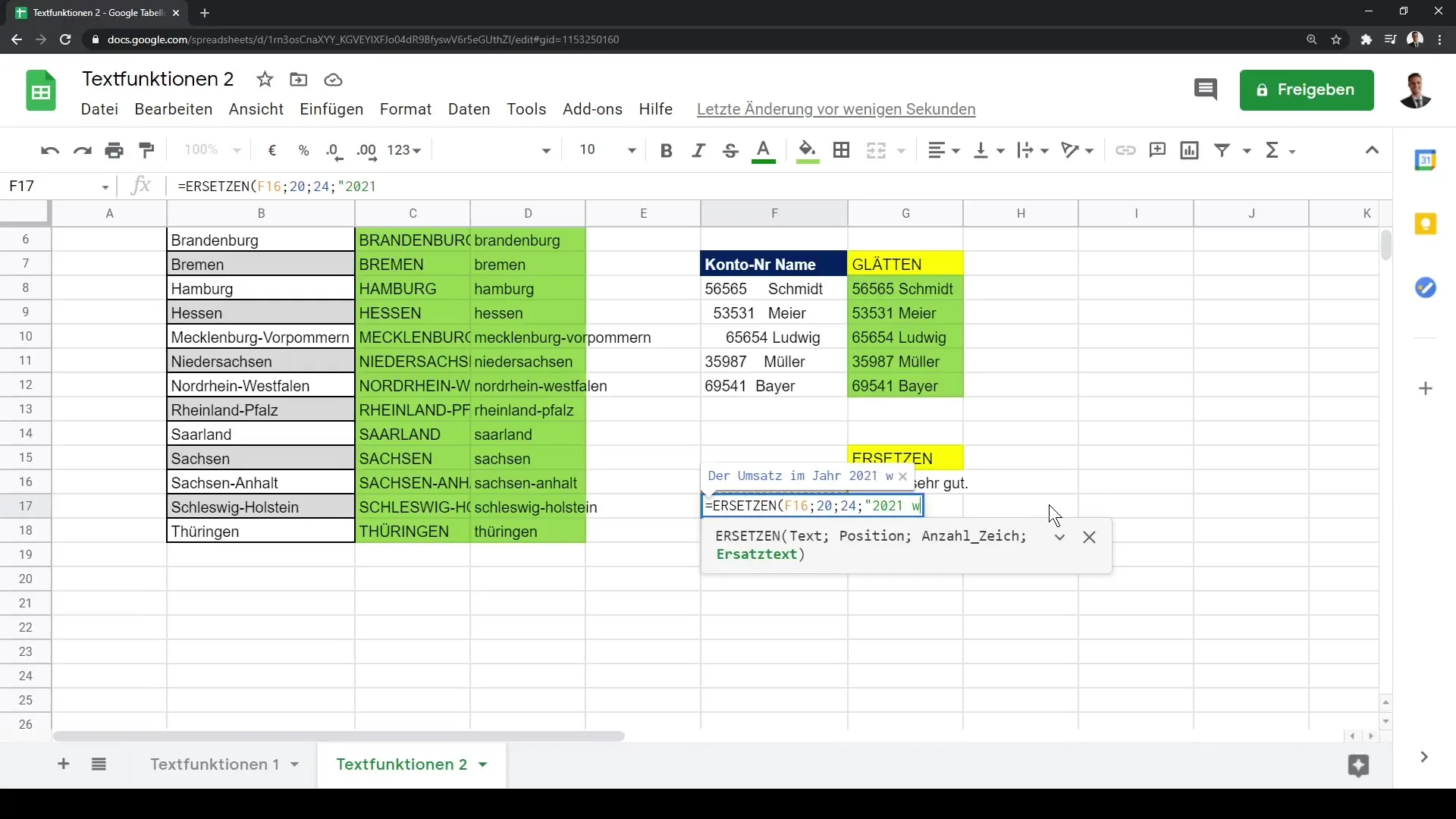
As a final step, let's look at the REPLACE function, which allows you to replace a specific word in a text string with another. Suppose you want to replace the word "good" with "bad" in a sample text. Start by entering the function in cell F16:

=REPLACE("The revenue in 2020 was very good"; 20; 4; "bad")

Here, you provide the original string, the position where the replacement should start, the number of characters to replace, and the new word. This screenshot shows you how the function is applied:

Overall, in this session, you have learned about the various text functions in Google Sheets, including UPPER, LOWER, SUBSTITUTE, TRIM, and REPLACE.

Summary

In this tutorial, you have learned how to use advanced text functions in Google Sheets to manipulate and customize data. The functions presented improve both your efficiency and flexibility in dealing with data in your Google Sheets.