Google Sheets Tutorial: Data analysis with Index and Match

In this tutorial, we delve deeper into Google Sheets and focus on the INDEX-MATCH function. After you are already familiar with the VLOOKUP function, in this lesson you will learn how to work more effectively with data in Google Sheets using Index and Match, especially when it comes to comparing and extracting information between different worksheets or tables. By utilizing these functions correctly, you can significantly improve your analysis and optimize your workflow.

Key Insights

The combination of the INDEX and MATCH functions allows you to efficiently retrieve data from large tables by specifying the position of a value in a matrix. This is particularly useful in extensive datasets and for cross-referencing workbooks.

Step-by-Step Guide

Step 1: Understanding the Index Function

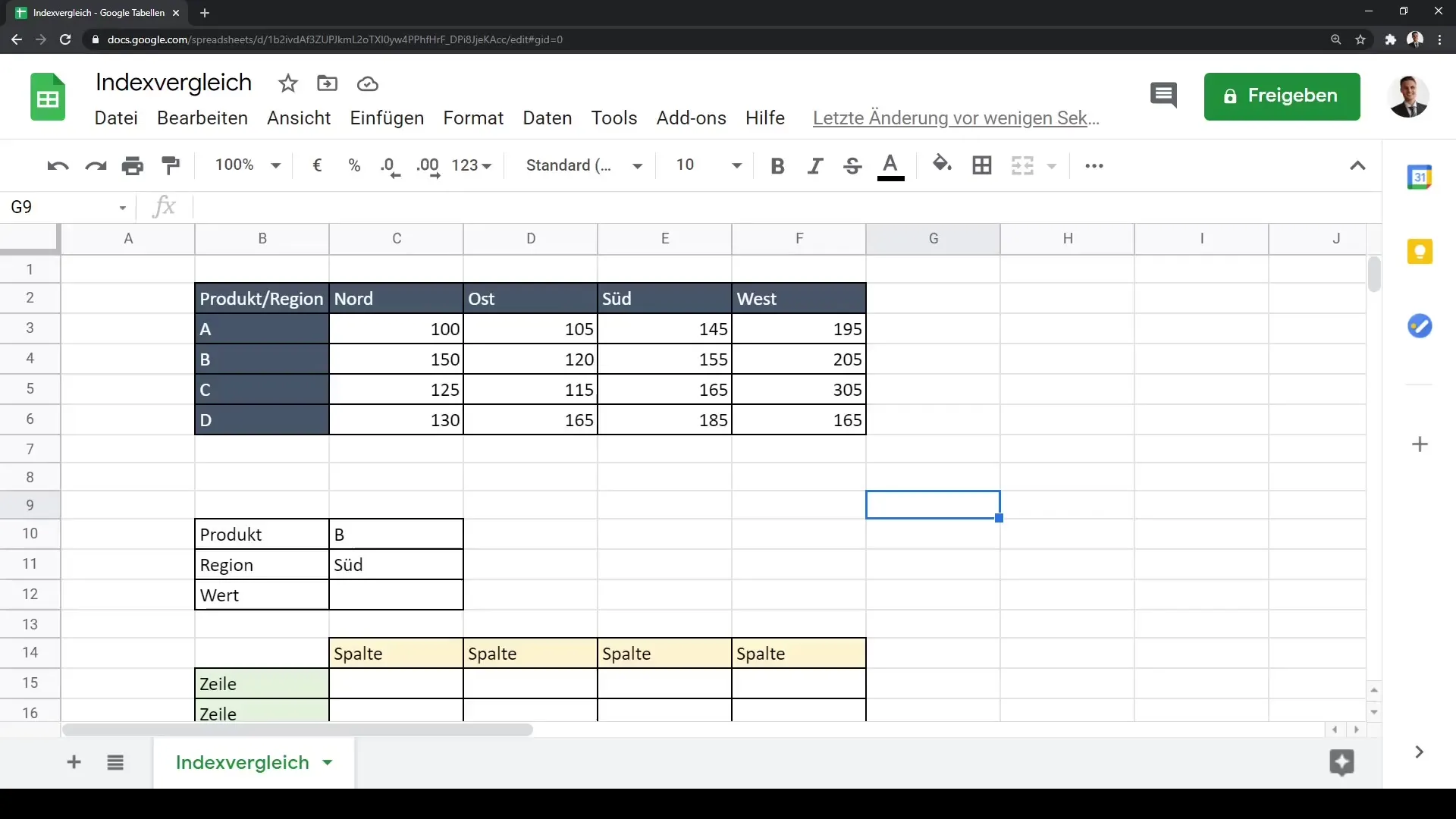
In order to understand the Index-Match function, it is important to first look at the INDEX function. This function returns the content of a cell in a specific range defined by row and column offsets. Essentially, you first select the target range from which you want to query data. A matrix would be helpful in this case, where the data is broken down by product areas and sales regions.

Step 2: Syntax of the Index Function

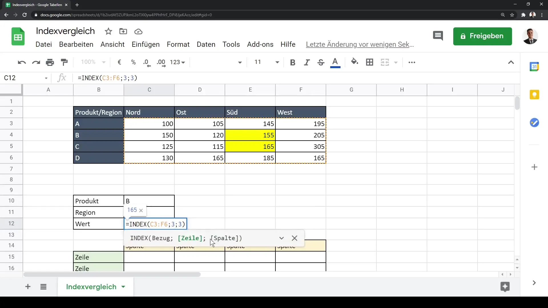
In this step, we will look at the syntax of the INDEX function. You must first set the reference, i.e., the cell range, and then select the specific coordinates. If you enter the example with coordinates 1 and 1, you will get the number 100 back, which is located in the sales region "North" and product area "A".

Step 3: Using Comparison Coordinates

Now we will adjust the coordinates and change them, for example, to 2 and 1. This change results in you getting the number 150 back, which is reflected accordingly in the table. With this method, you work like in the game "Battleship", by specifying the exact positions you want to query.

Step 4: Introducing the Match Function

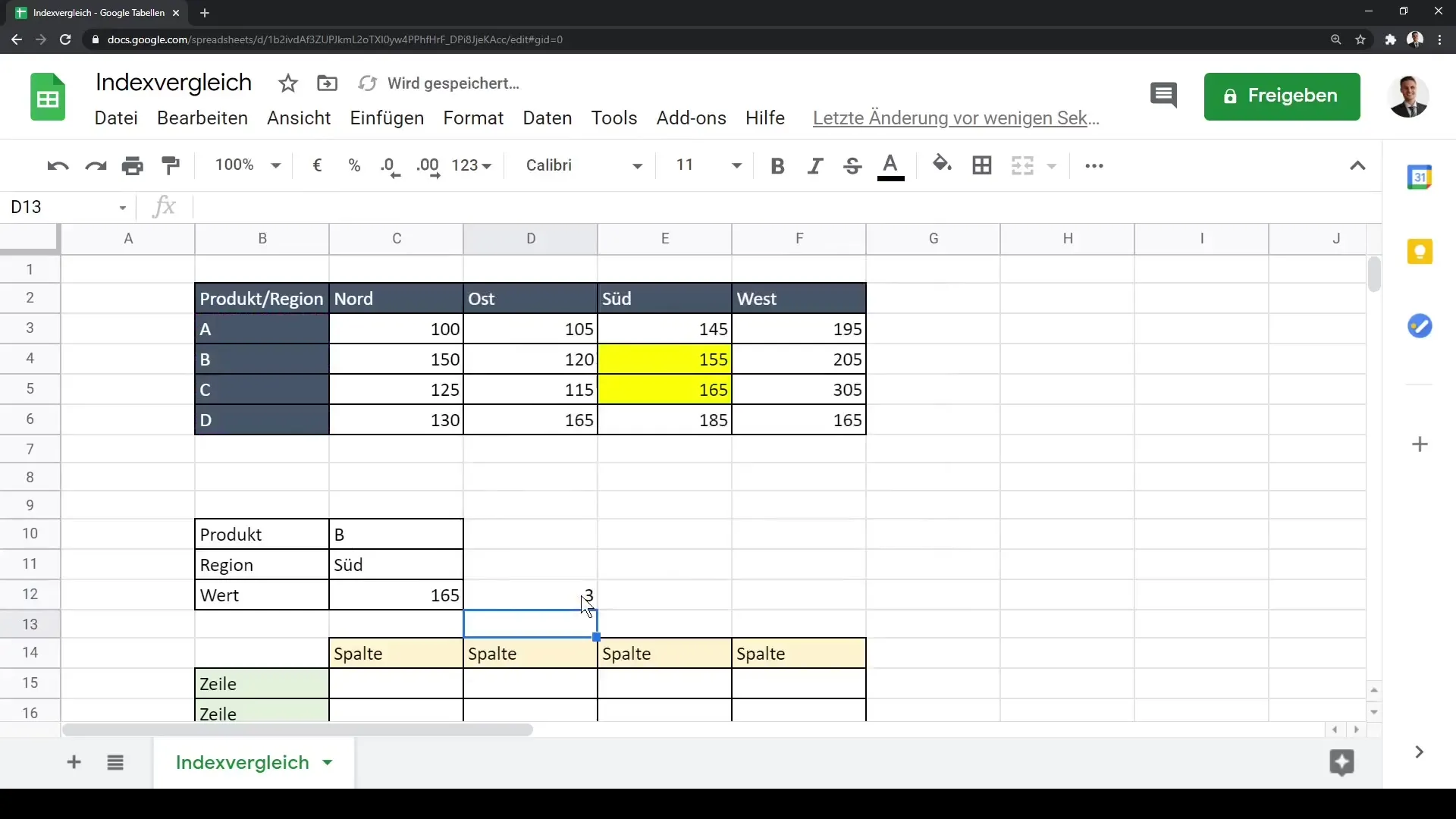
In the next step, we explain why we talk about "Index-Match". In addition to the INDEX function, there is also the MATCH function, which returns the position of an element in a specific range. By specifying a reference range from A to D, you can easily find where, for example, the product "A" is located in this matrix.

Step 5: Combining Index and Match

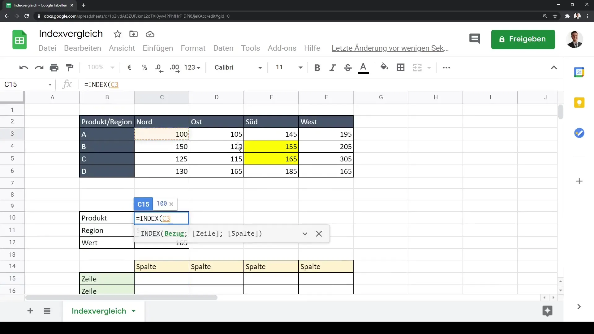
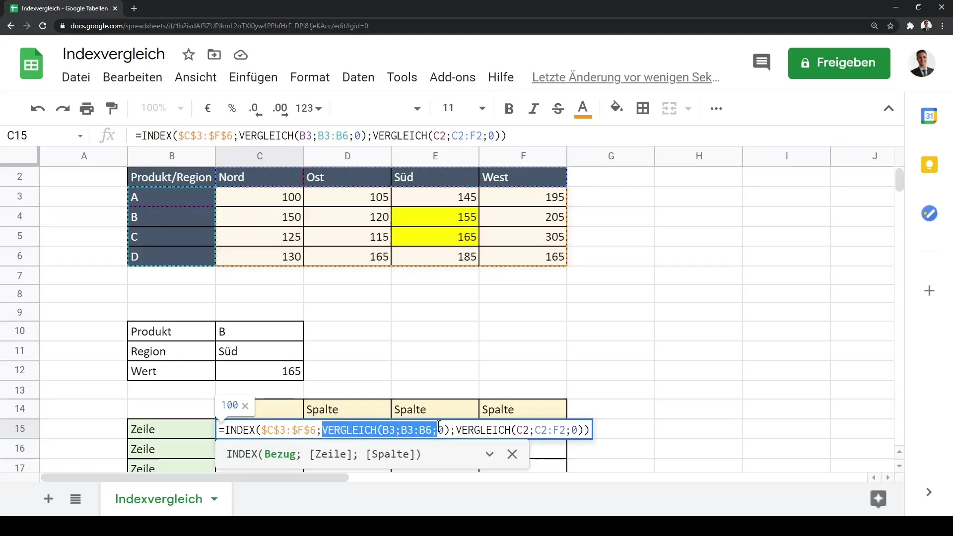
This is where the interaction of INDEX and MATCH comes into play. After determining the position of a value (e.g., "A") in the matrix, you can combine it with the INDEX function to retrieve the corresponding cell content. In essence, you take the results from the MATCH function and use them as coordinates for the INDEX function.

Step 6: Setting Fixed References

To further optimize your work, you should set fixed references. If you set the entire reference matrix with F4, you can easily drag the formulas down and to the side without manually adjusting the formulas. This greatly facilitates the application and work with datasets.

Step 7: Adjusting the Formulas

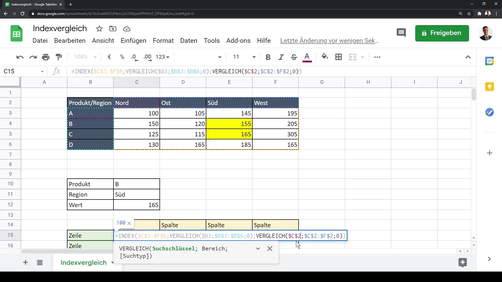
Now we will adjust the formulas so that the correct references are maintained as you drag the formulas down. By adjusting the dollar signs in the references, you can ensure that the variable parts of the formula are correctly updated when dragged.

Step 8: Application and Transposition

Once everything is set up, you can drag the formulas to the end of your table. This will enable you to efficiently extract all desired values and help you transpose the data if necessary. The INDEX MATCH function significantly simplifies and speeds up data analysis.

Summary

In this guide, you have learned how to use the INDEX and MATCH functions in Google Sheets to efficiently compare and retrieve data. Combining these functions allows you to work flexibly and dynamically with your datasets.