Cell formatting in Google Sheets - The ultimate guide

In this tutorial, you will learn how to effectively format cells in Google Sheets. Whether it's about border lines, fonts, color changes, or adjusting number formats - here you will get a complete overview of the possibilities for cell formatting of your data. A well-structured table not only conveys information precisely but also looks appealing. Let's get started right away!

Key Takeaways

• Add and adjust border lines
• Change background and font colors
• Adjust fonts and sizes
• Display numbers formatted (currencies, percentages, etc.)
• Apply conditional formatting
• Create merged cells and change alignments

Step-by-Step Guide

To start formatting your table, first select the entire table. You can do this by hovering your mouse over the top row and left column and then clicking on the square in the upper left corner. This will activate the complete table.

After selecting the table, you will see a variety of tools in the menu bar at the top that you can use to edit your data. Think of these tools as a workshop where you select the right instruments for editing your content.

One of the first things you can do is add border lines. To do this, click on the "Borders" icon in the toolbar. There are different options for border lines, but here we will initially choose the option for all borders to create a complete border around the cells.

After adding the border lines, you can change the color of the lines. To do this, select the appropriate color menu and experiment with different colors, such as a bold blue or a dark red. You can customize the border to your liking.

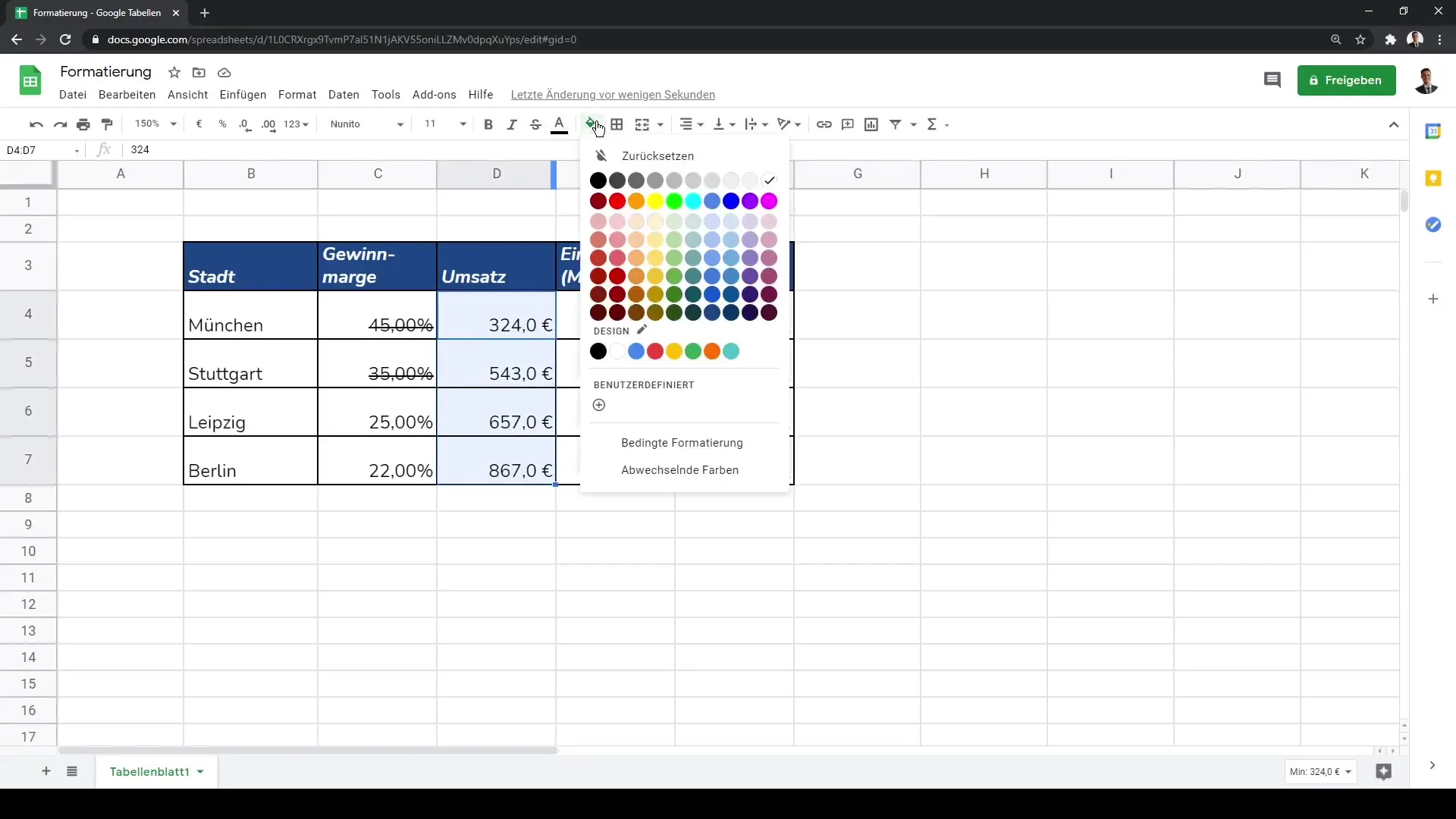
In addition to border lines, it is important to also change the background color of your cells. To do this, click on the fill color and choose a color that you like. We recommend a dark background, such as blue, with white font color for better readability.

Now you can adjust the font in your cells. Highlight the desired text and then select the font from the menu. "Arial" is set by default, but you can change it to another font, such as "Nunito," to add variety.

Another possible adjustment is changing the font size. Select the cell or text and change the size to make it more readable. A larger font size can help highlight important data.

You can also format text as bold or italic to emphasize certain entries. The keyboard shortcut "Ctrl + B" makes the text bold, while "Ctrl + I" italicizes it. This significantly improves the clarity of your table.

Keep in mind that sometimes the entire text in a cell is not visible. Here you can enable text wrapping so that long texts are distributed over multiple lines. This is done by selecting the cell and choosing the text wrapping option.

Another important point is number formatting. For example, you can set the number of decimal places displayed for numbers. Click on the desired cell or range of numbers and select the option for the number of decimal places.

You can also add new columns if you want to represent more information, such as sales figures. You can also display these numbers in currency format to clearly identify them. Manage the decimal places according to your needs.

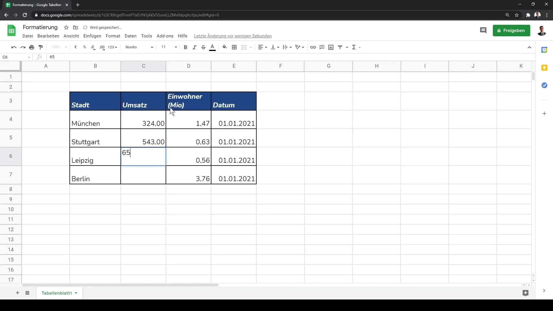
For a comprehensive overview of the data, profit margins can also be added as percentages in a column. Use the percentage formatting option to design this column accordingly and create professional reports.

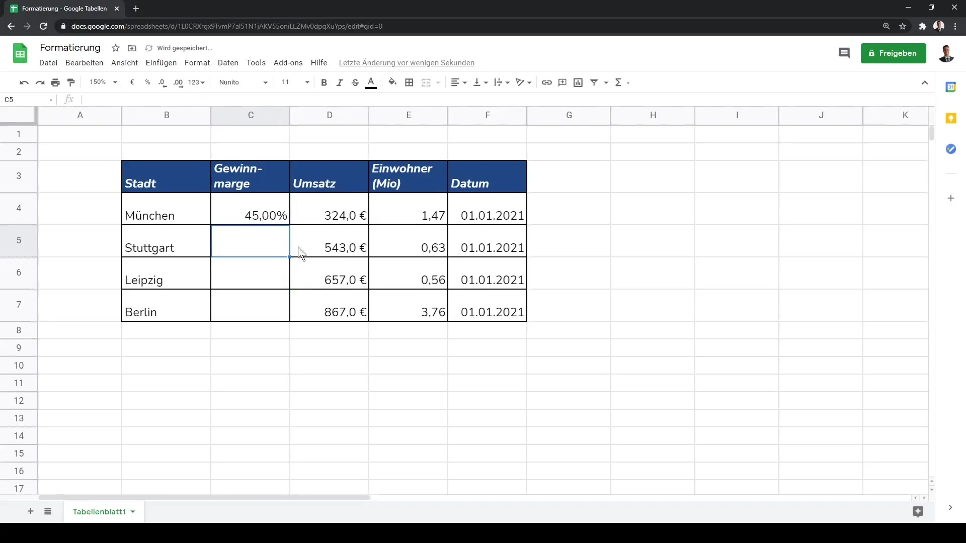
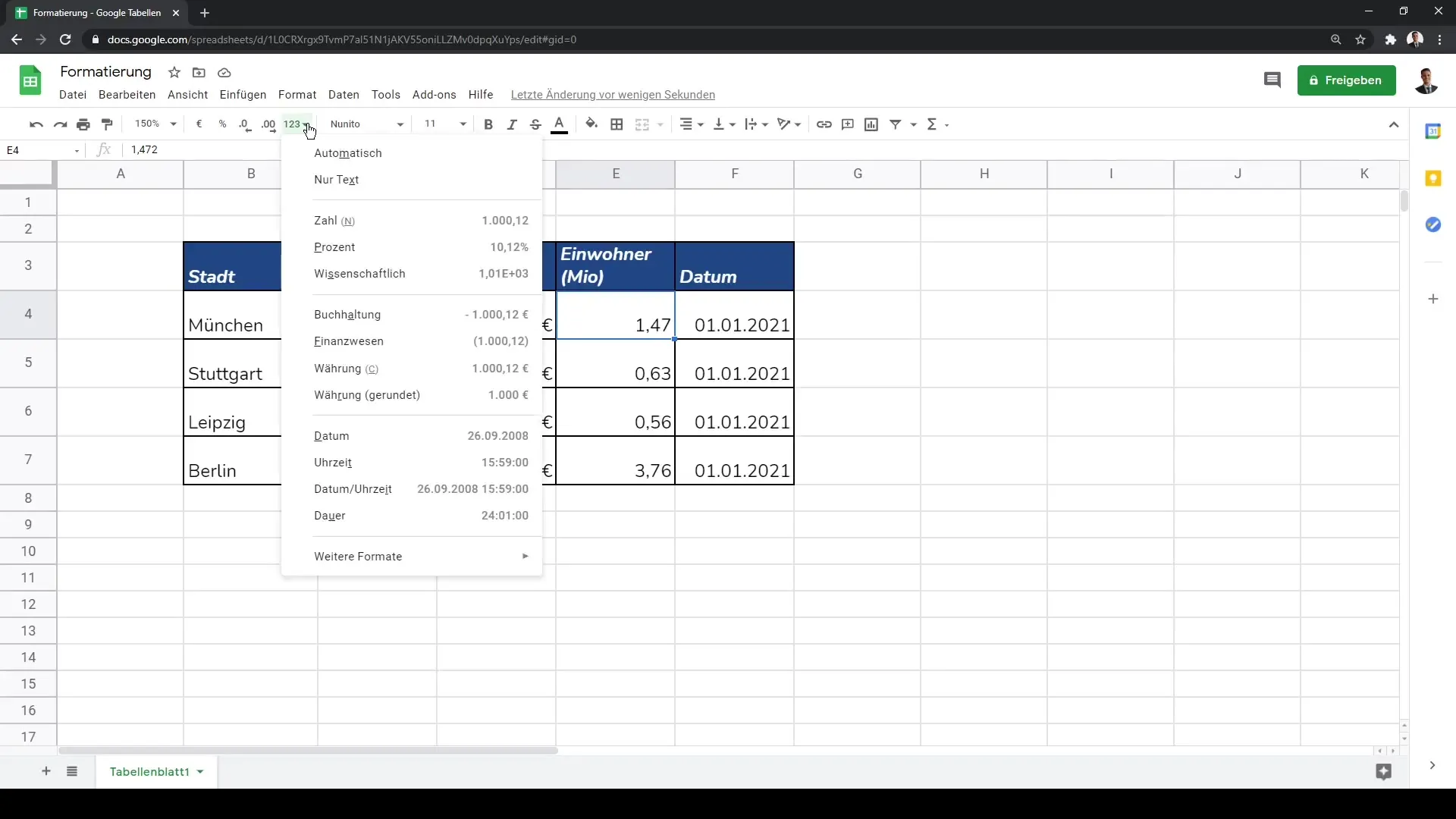
There are many more formatting options you can use. Simply click on "More formats" in the menu, where you will find various options such as scientific notation, accounting formatting, and various currency formats.

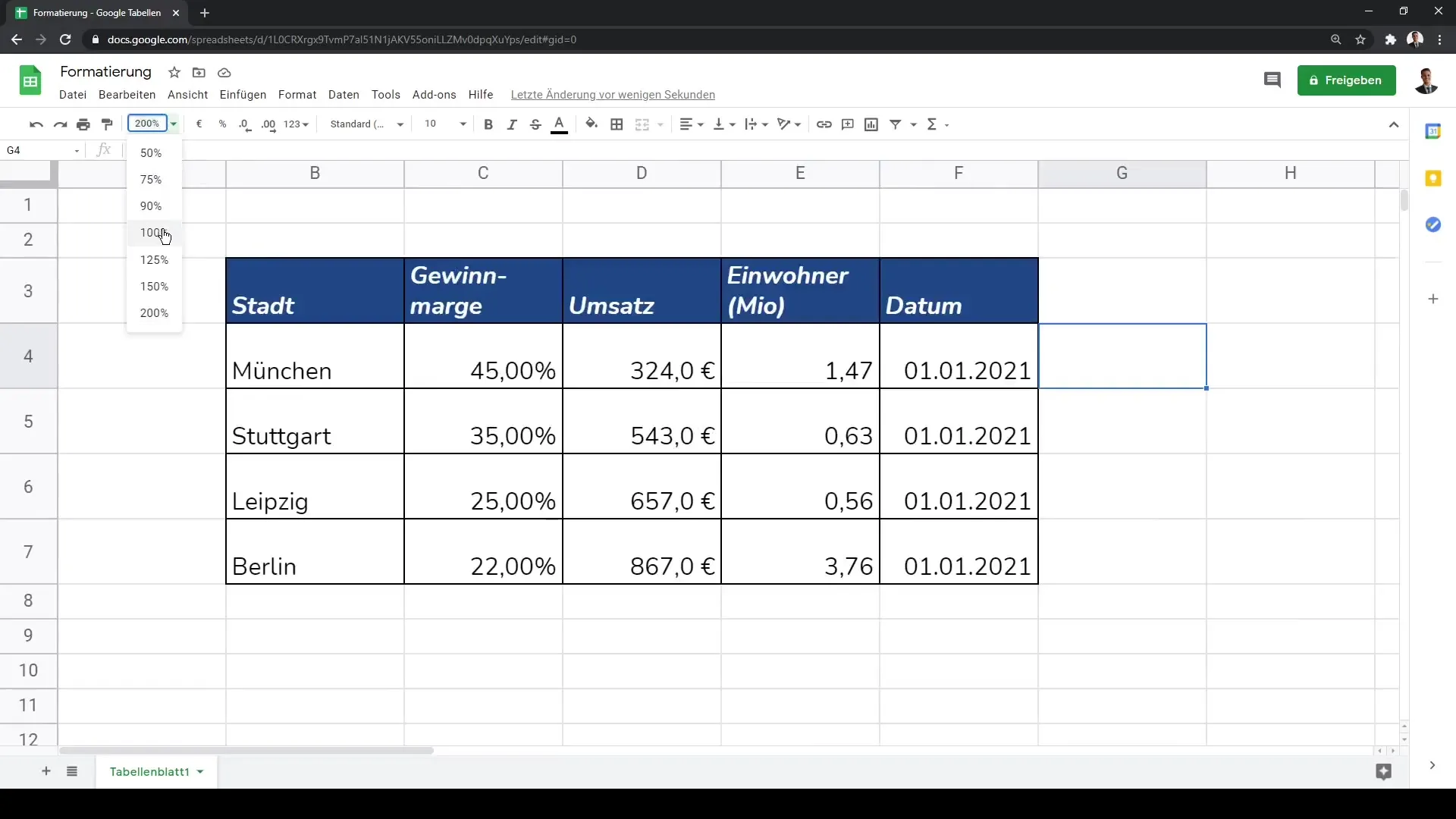
To customize the view of your table, you can also change the zoom of the worksheet. This is particularly helpful to maintain an overview. Simply go to the zoom settings in the toolbar.

In addition to the basic formatting functions, you can also use conditional formatting to display certain numbers in different colors, depending on whether they are large or small. This greatly improves the visual representation of your data.

If you want to merge cells, simply select the appropriate cells and use the "Merge cells" function. This is particularly useful if, for example, you want to display a company name across multiple cells.

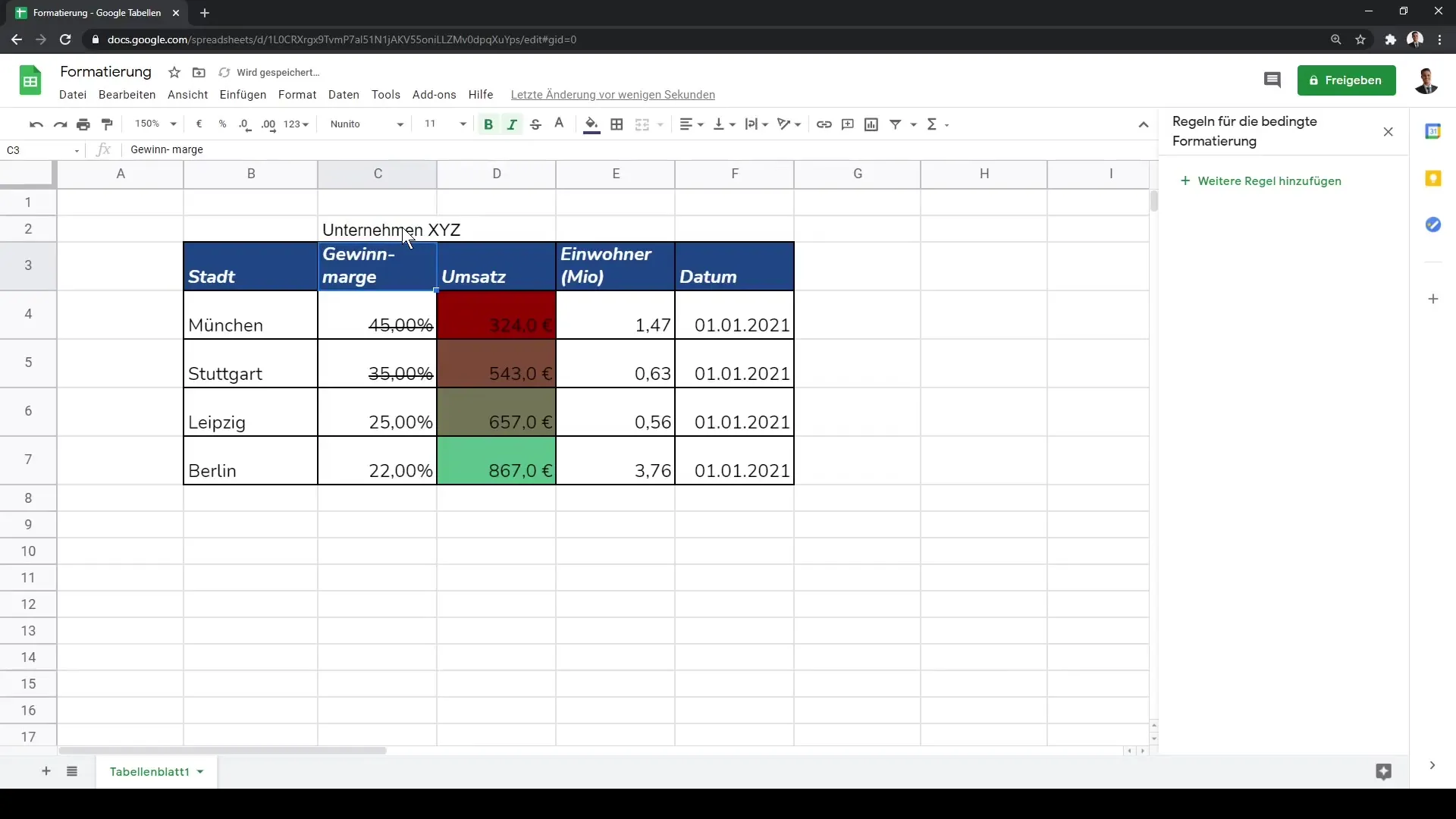
To optimize the readability and layout of your table, you can also change the alignment of the cells. Try out different alignment options and find the best one for your table.

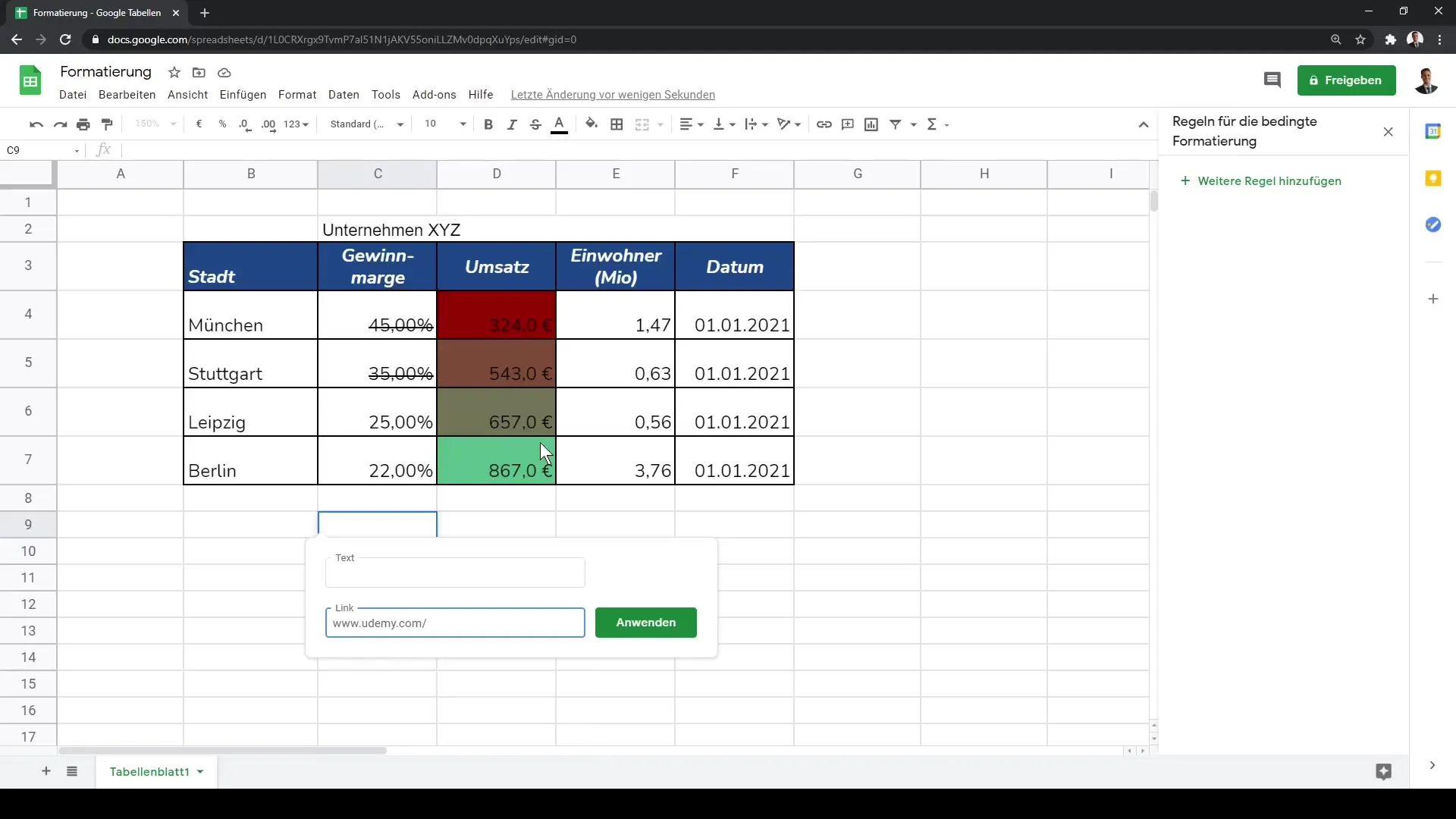
Furthermore, it is also possible to insert links into your cells. This is particularly helpful if you want to access external websites or documents. Remember to enter the URLs correctly so that they function.

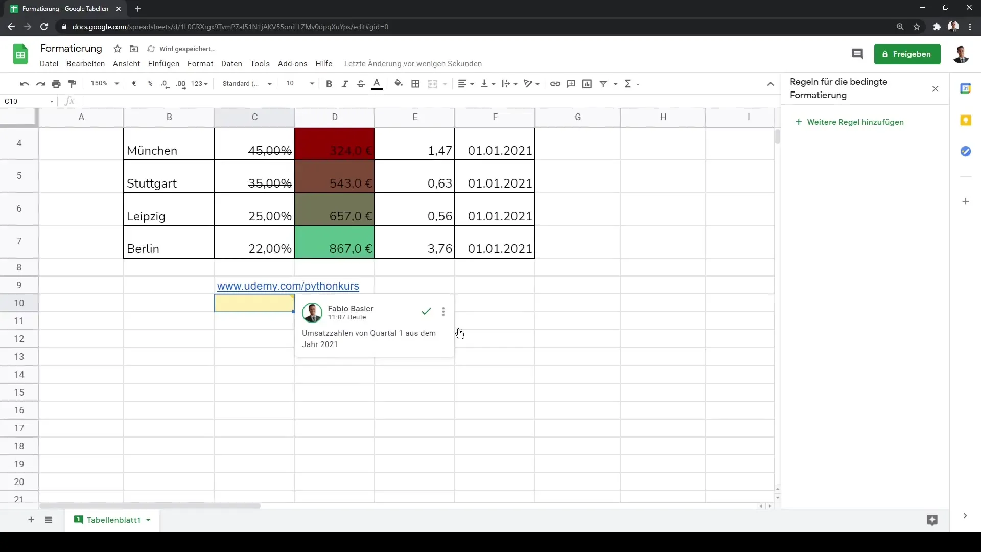
You can also add comments to the cells that are visible to other users who open the file. This is especially useful for teamwork and providing relevant information or notes.

These steps cover the basic cell formatting functions in Google Sheets. Use these techniques to make your tables attractive and informative.

Summary

In this guide, you have learned how to format cells in Google Sheets by adding borderlines, changing fonts, formatting numbers, and much more. The targeted application of these formatting options helps you present your data more clearly and attractively.