Welcome to this comprehensive tutorial on optimizing the view and layout in Google Sheets. In this lesson, you will learn how to customize your tables to achieve the best user experience. We will explore various features that allow you to present your data clearly and attractively.
Key Takeaways
In this course, you will learn how to show or hide gridlines, freeze rows and columns, set up protected areas, manage the formula bar and status bar, and enhance the layout of your table. By the end, you will be able to optimize your Google Sheets documents.
Step-by-Step Guide
1. Adjust Gridlines
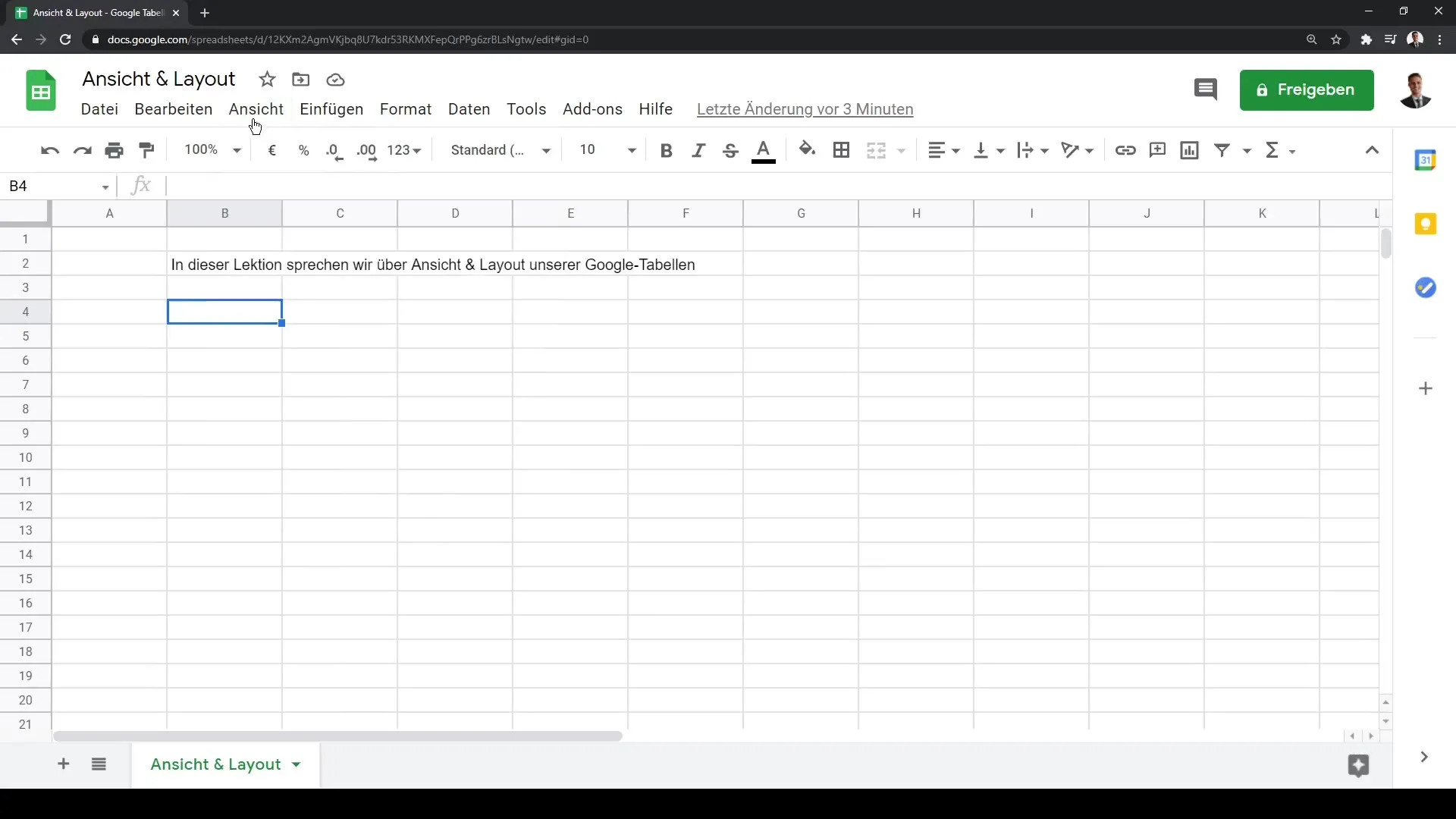
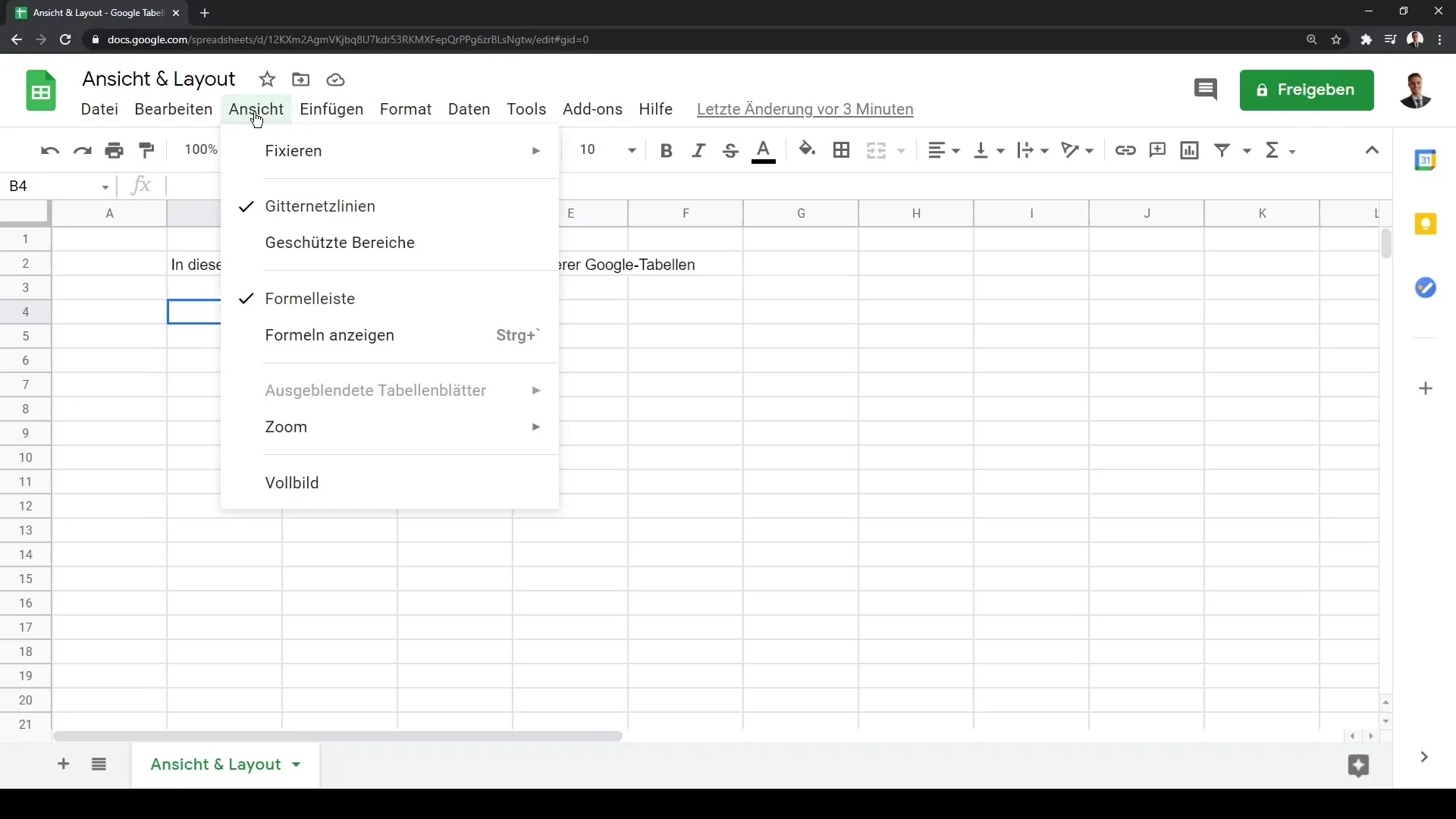
One of the first steps in personalizing your Google Sheets is adjusting the gridlines. By default, these lines are visible, but you can hide them to get a clearer view of your document. To do this, go to the "View" tab and uncheck "Gridlines".
2. Freeze Rows
To maintain clarity while scrolling through large amounts of data, it is advisable to freeze relevant rows, especially headers. You can do this by clicking on the "View" tab again and selecting "Freeze." Here, you have the option to freeze a specific row or up to the selected row. Choose the appropriate option for the row you want to freeze.
3. Freeze Columns
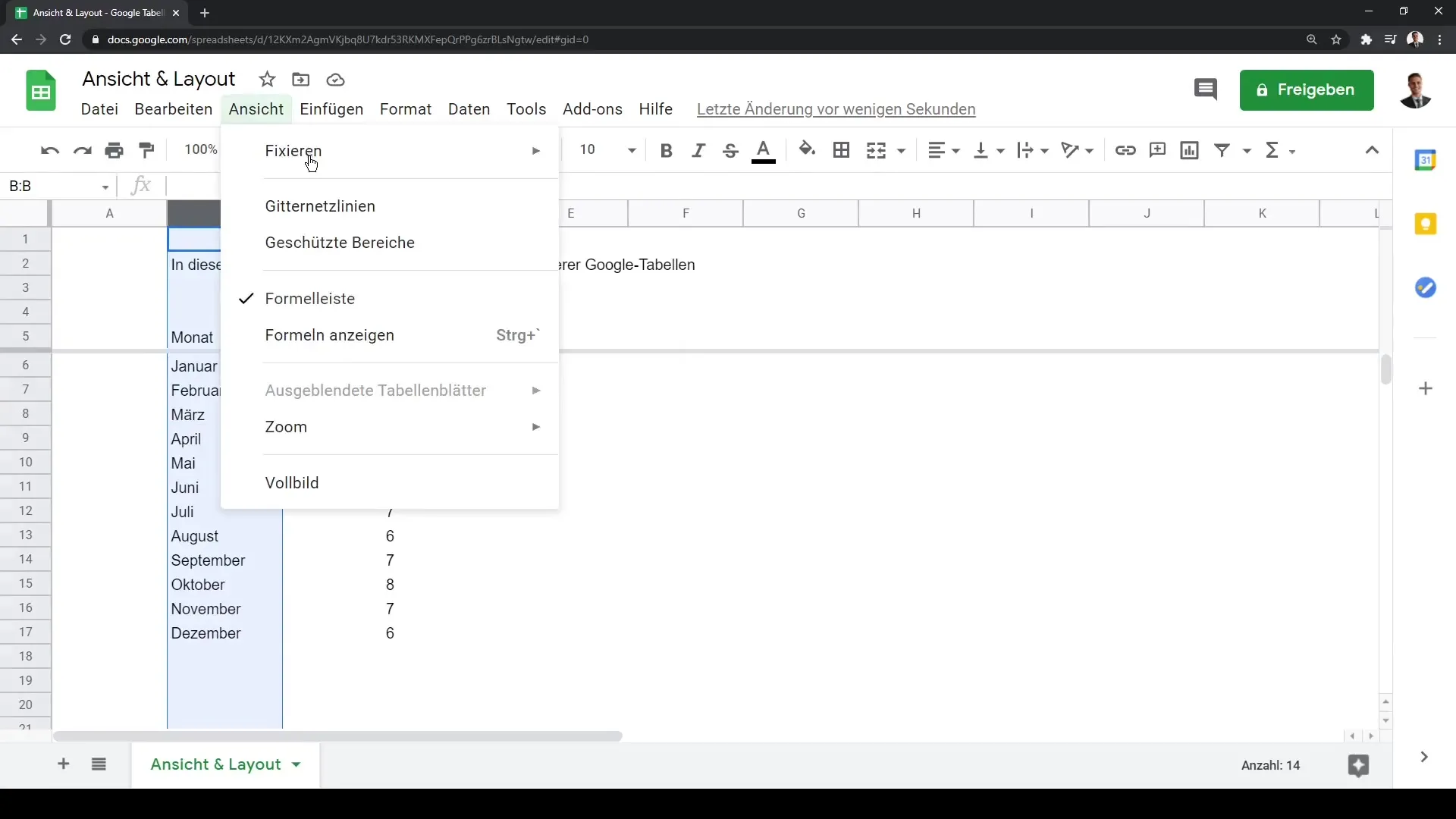
Similar to freezing rows, you can also freeze columns. Go to the "View" tab and click on "Freeze" to freeze a column up to the selected column. This is particularly useful when you have large tables with many columns and want the first columns to remain visible.
4. Set Up Protected Areas
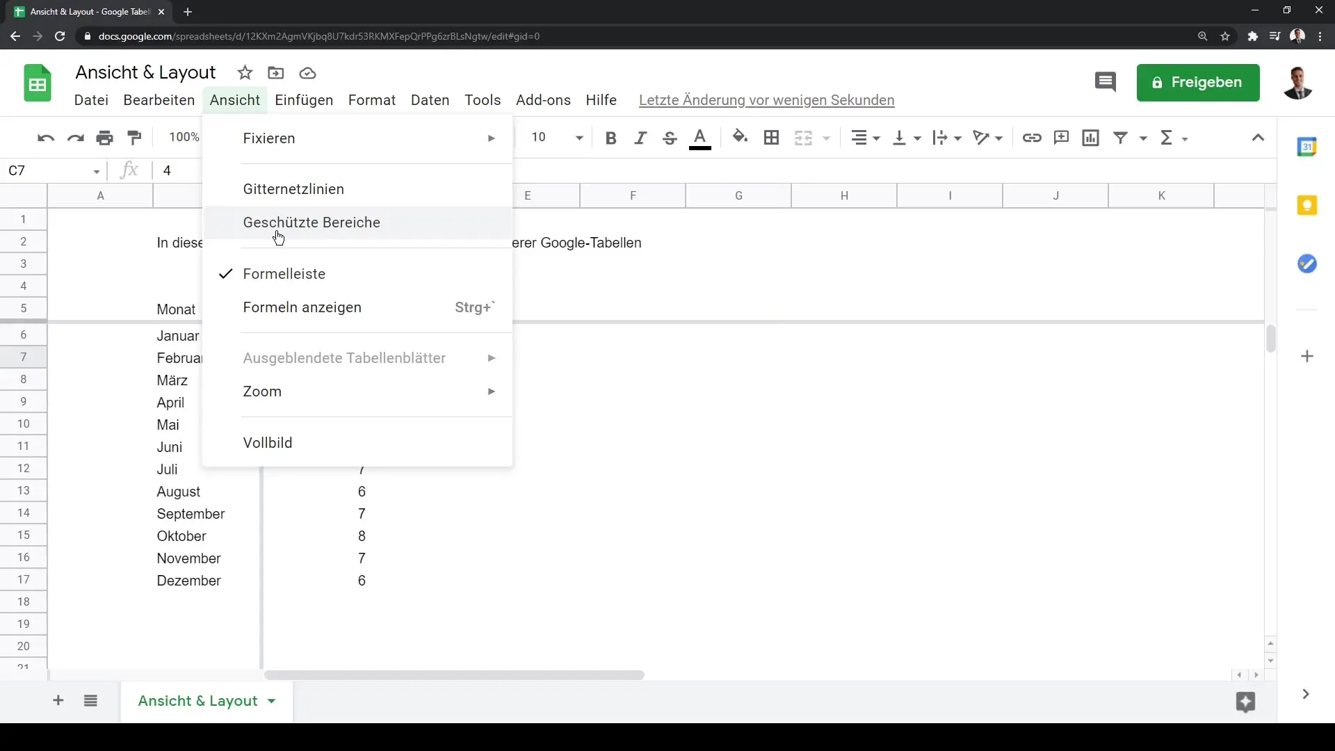
Do you want certain cells to be uneditable? Go to "View" and select "Protect selected cells." You can then set which areas are visible but not editable for other users. This is especially important when sharing a table with colleagues and want to ensure that certain data is not altered.
5. Manage Formula and Status Bar
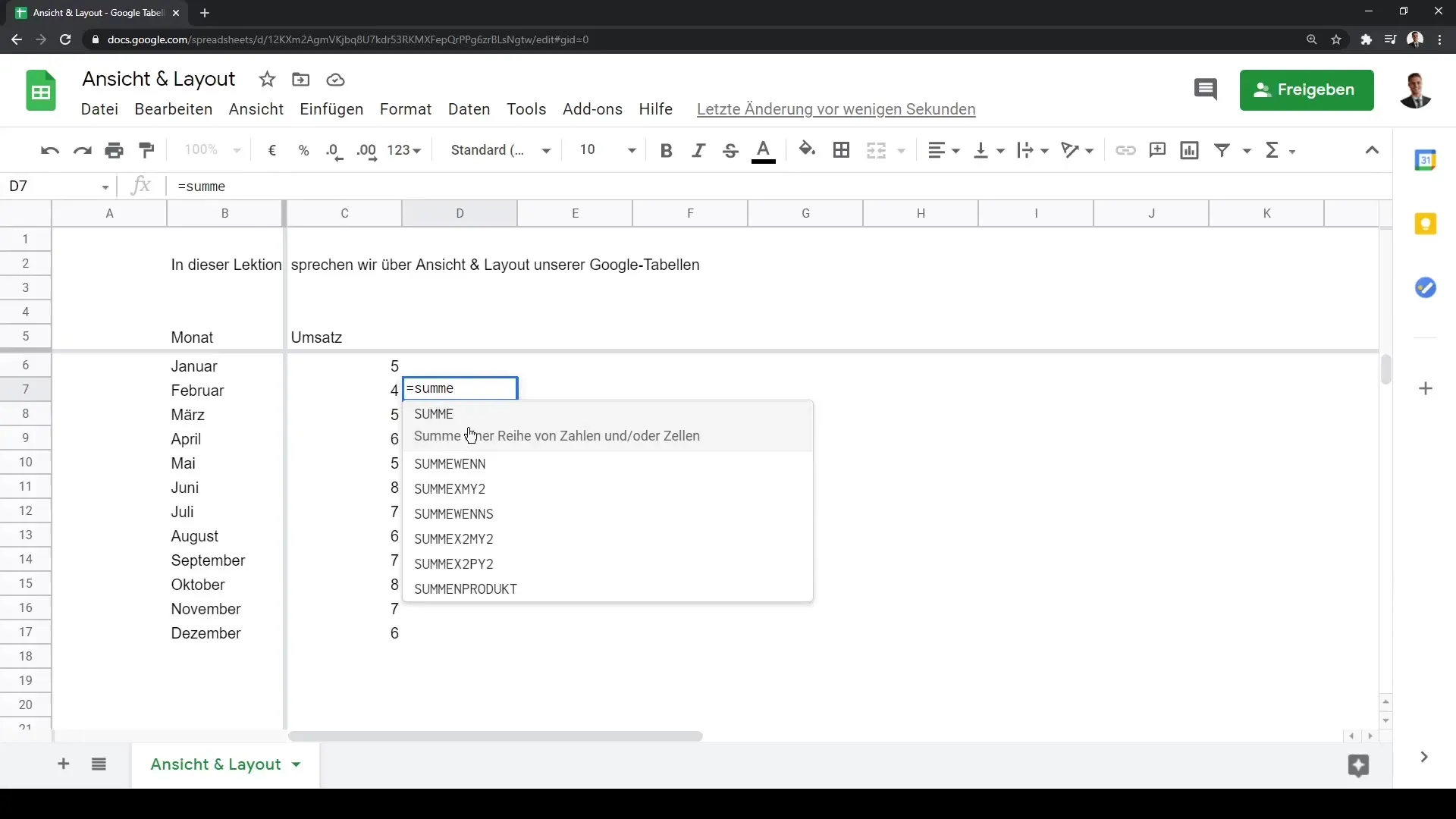
Another useful function is controlling the formula and status bar. You can decide whether the formula bar should be enabled or disabled. Also, you can choose whether you want to see the calculation results or the actual formulas. You can find these options under the "View" tab.
6. Zoom Adjustments
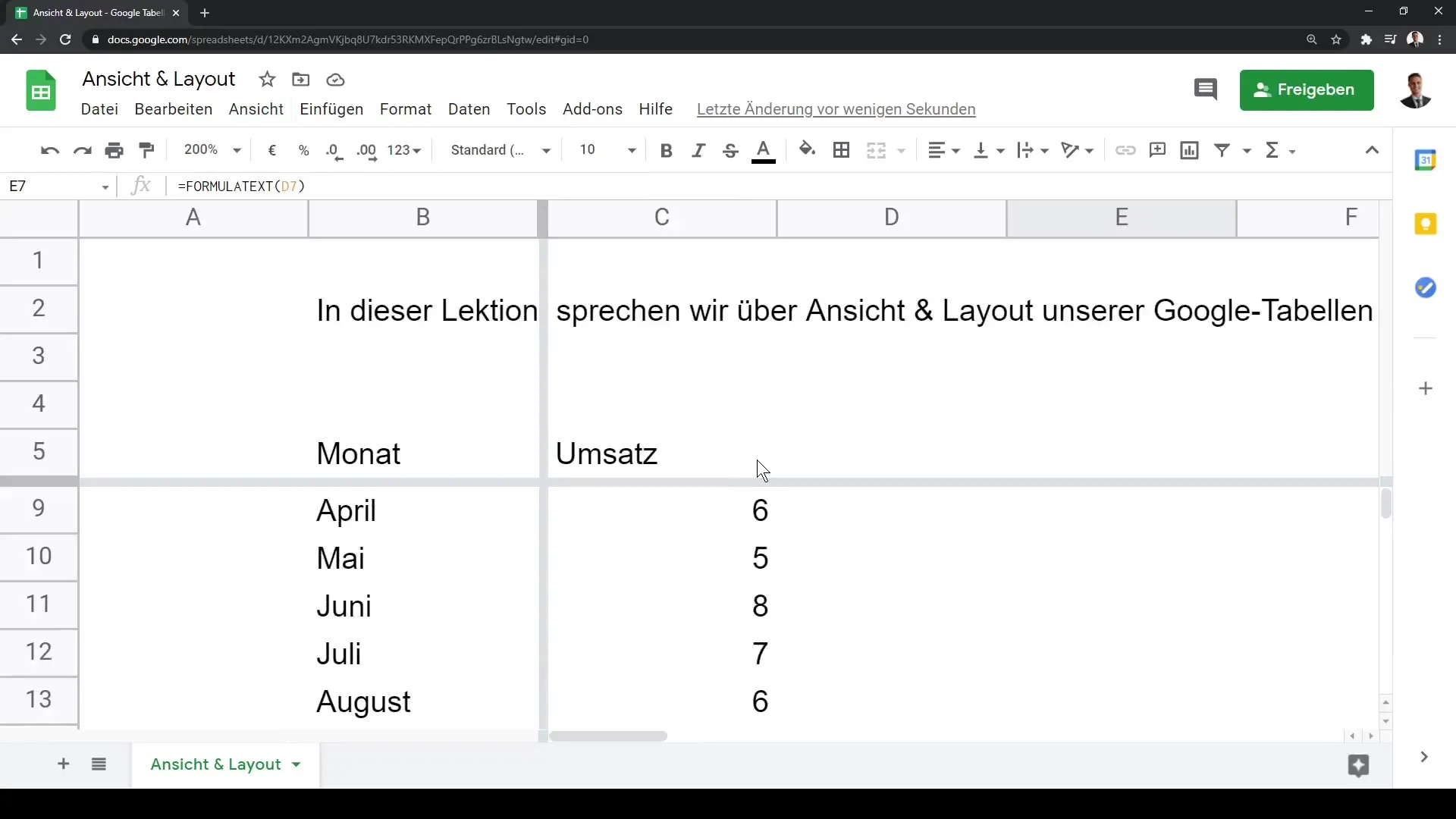
Another important tool is the zoom function. You can zoom in or out the entire document to see details better or get a better overview. You can do this through the zoom adjustments in the top right corner of the user interface. For example, you can set a zoom of 100%, 125%, or even 200%.
7. Use Full-Screen Mode
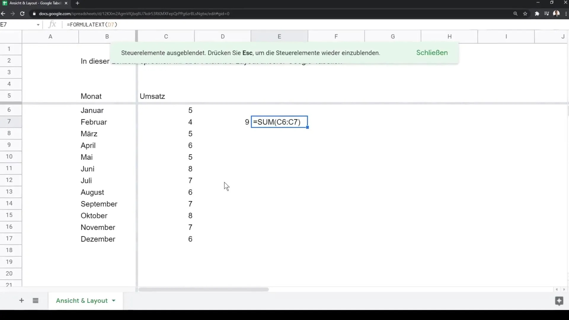
If you want to concentrate more on your work, you can also activate full-screen mode. Go to "View" and select "Full Screen." To exit full-screen mode, simply press the "Escape" key.
8. Customize Design
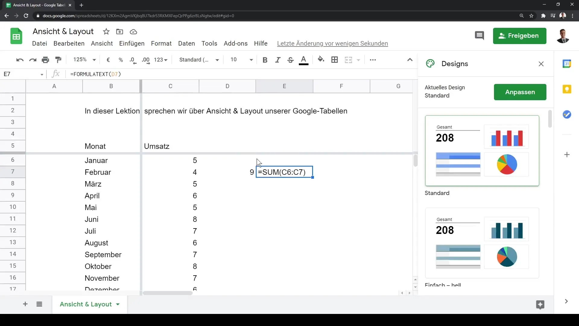
The aesthetic design of your Google Sheets is also crucial. You can customize the design of your table by selecting various layouts in the "Format" tab, such as "Default," "Simple Light," or "Streamline."
9. Formatting Cells
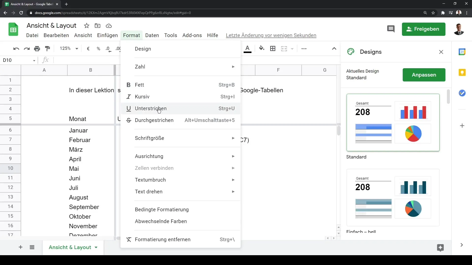
Also consider the options for formatting cells. You can display text in bold, italics, or underlined, change the font size, and much more. This helps to highlight important information and improve readability.
Summary
In this guide, you have learned how to optimize the view and layout of your Google Sheets documents. From adjusting gridlines to fixing rows and columns to setting up protected areas - you now have the tools to design your tables as you wish.
Frequently Asked Questions
How can I hide the gridlines?Go to the "View" tab and uncheck "Gridlines".
How do I fix a row in my table?Select "View", click on "Freeze" and choose the option for the desired row.
Can I create protected areas in Google Sheets?Yes, go to "View" and choose "Protect Selected Cells" to lock certain cells.
How can I change the zoom settings?You can find the zoom function in the top right corner of the user interface, where you can select the desired percentage.
Can I customize the font in the cells?Yes, under the "Format" tab you can customize font, size, and formatting such as bold or italics.
