Google Sheets: Conditional formatting of cells made easy

In this guide, you will learn how to use conditional formatting in Google Sheets to visually and clearly style your data. Conditional formatting allows you to highlight data visually, so you can quickly see how your numbers are developing. Whether you are analyzing monthly profits, revenue, or expenses – through suitable color design, you can immediately recognize patterns and deviations. Follow the step-by-step guide to manage your data more effectively.

Main Takeaways

Conditional formatting helps to visually represent data.

1. You can use different color scales to easily identify profits and losses.
2. Empty cells or specific values can also be highlighted.
3. It is possible to apply multiple rules for different data ranges.

Step-by-Step Guide

Start by opening your Google Sheets file where you want to apply conditional formatting. Make sure that all data has already been entered, especially the financial data you want to analyze.

When you are in the spreadsheet, look for the "Format" tab in the top menu. Click on it to access the options.

Scroll down to "Conditional Formatting." When you click on that, a menu bar will open on the right side of your screen.

Now you need to select the range of cells you want to format. For example, you can choose the range from January to December for your profit numbers. Highlight the entire range you want to apply conditional formatting to.

Once the range is selected, click on "Fill color" and navigate to "Conditional Formatting." Here you can adjust the color scheme.

In the next step, add a formatting rule. There are various options; we will work with a color scale. Choose the color scale as we want to highlight profits visually.

You can set high profit numbers to be displayed in green and lower ones in red. This gives you an immediate overview of how good or bad the months are going.

There is a default color scale available that you can use directly. However, you can also define the values yourself and adjust the colors if you do not like them.

If you are satisfied with the default settings, simply click "Done." This will apply the color scale to the selected data.

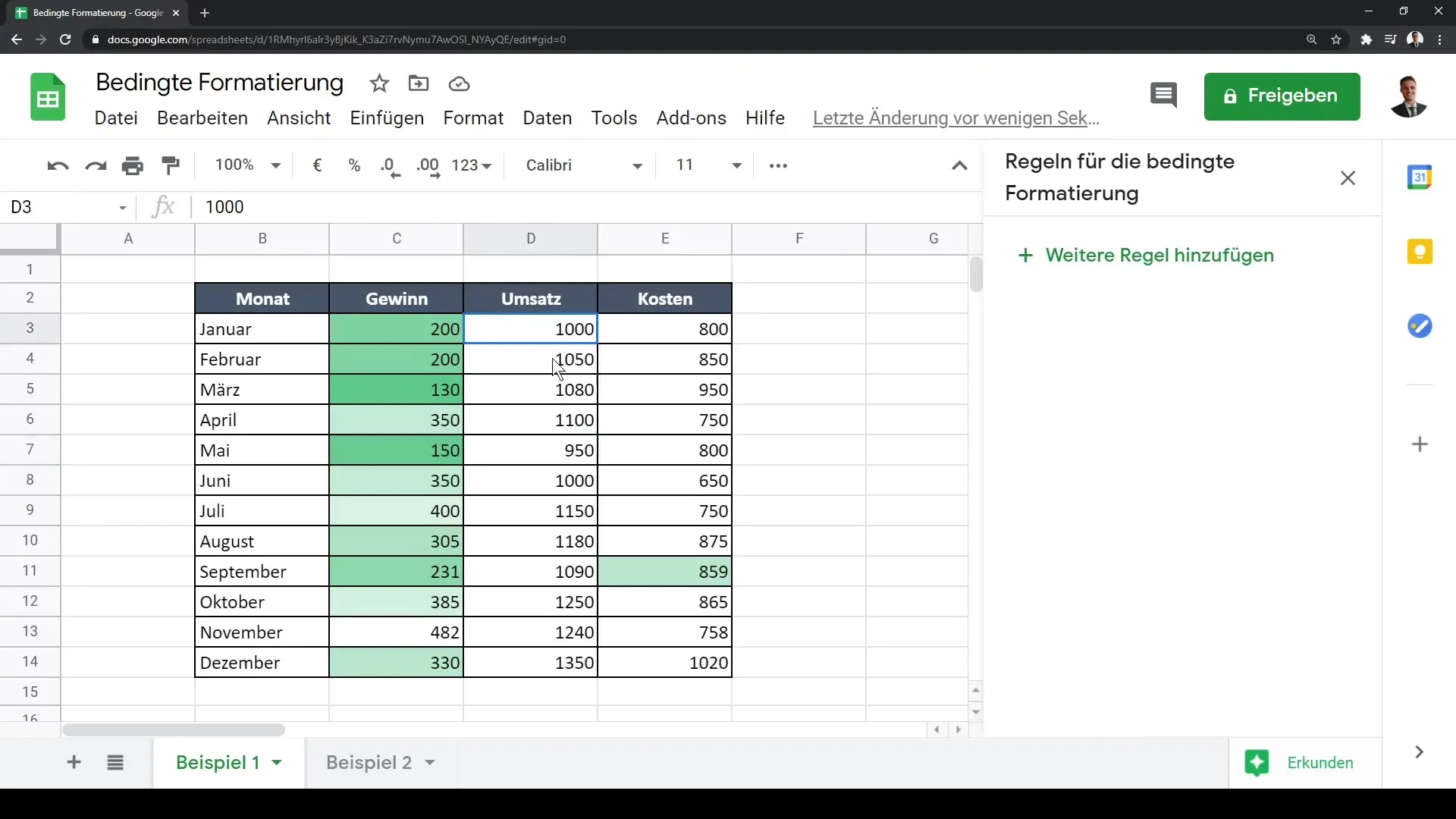
Would you like to format another dataset, for example, the revenues? Also select the relevant cell range here and go to conditional formatting again. Click on "Apply another rule."

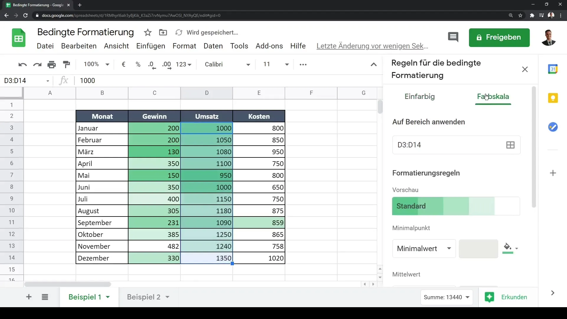
Repeat the steps for the color scale, but this time, we want to reverse the parameters: set the higher numbers to red and the lower numbers to green. This helps visualize the expenses.

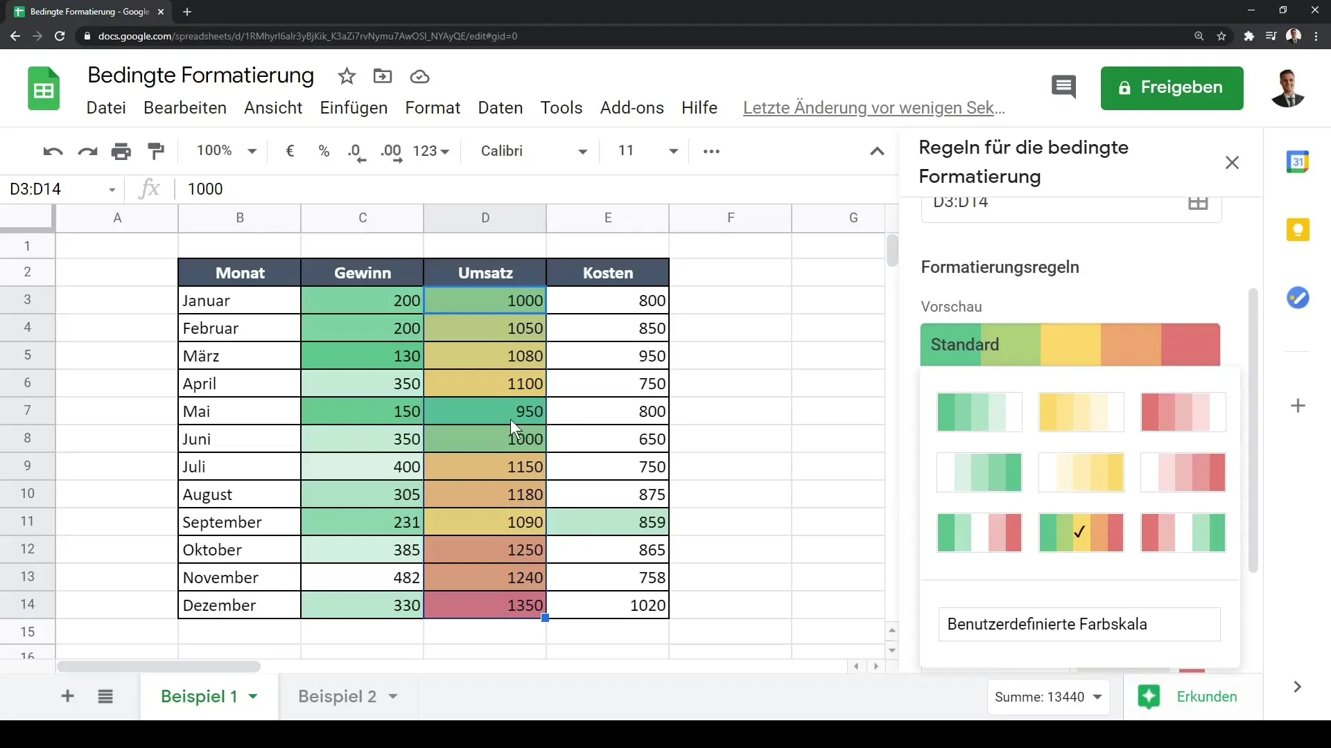
Before saving the new rule, remove the previous rule for revenue to avoid overlaps. Do this using the trash can symbol.

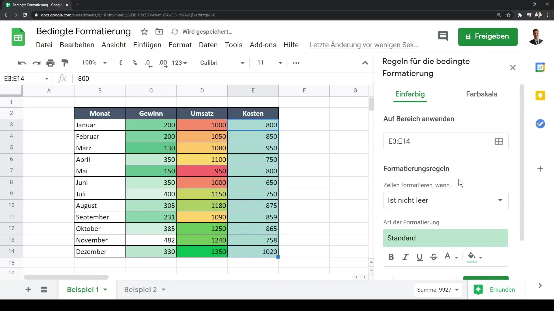
If you are happy with the settings, click "Done," and the rule will be applied immediately.

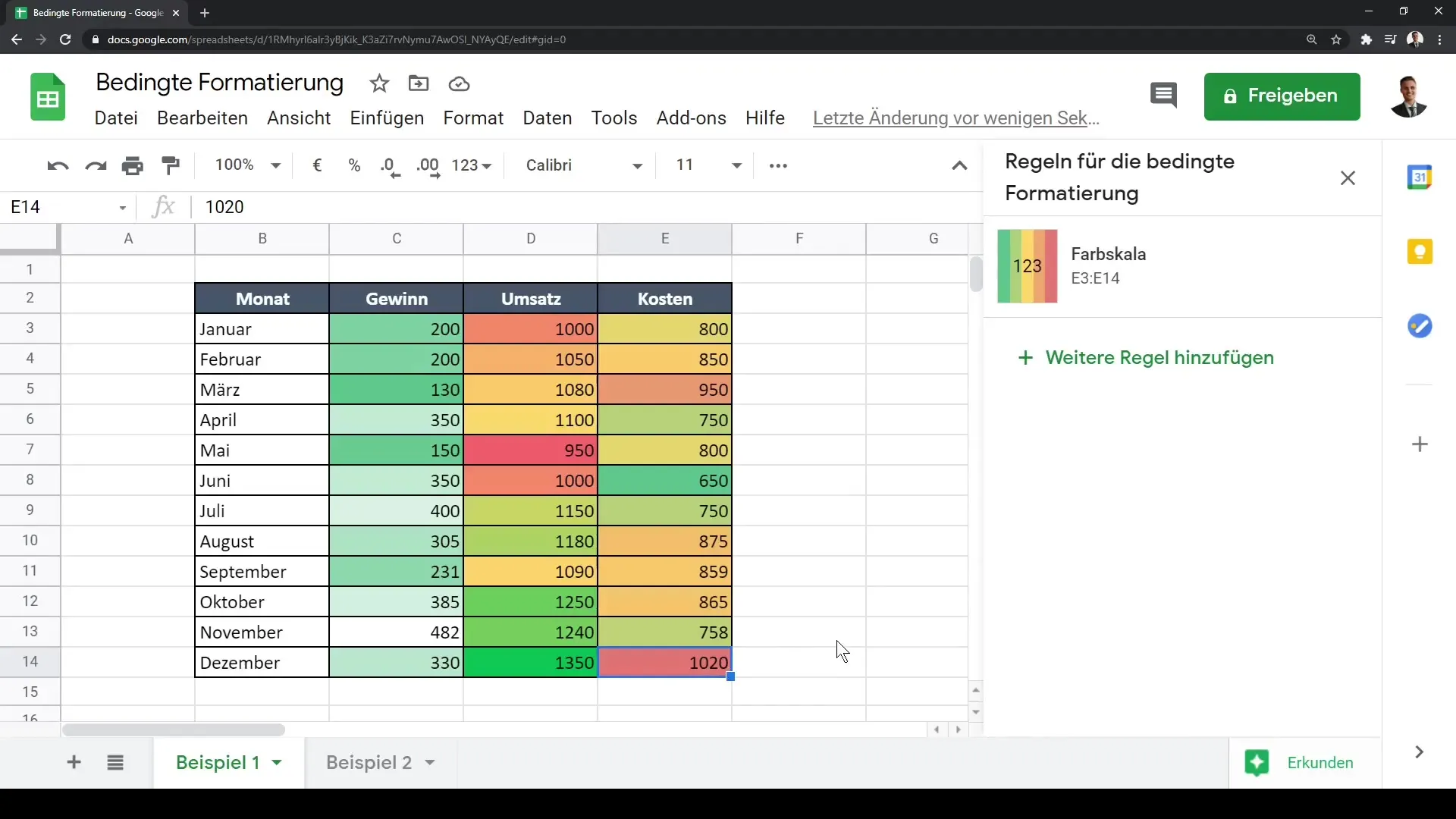
If you are working with large data sets, it can be helpful to make empty cells visible. Select the entire data range and go back to conditional formatting.

This time, select the rule "Cells that are empty" to, for example, color them black. This signals to you that data still needs to be entered here.

The same applies to other columns, such as revenue data. Make sure to apply the same rule here as well to ensure a consistent format.

Finally, you can use the color scale in another column to also set visual warning signals there. Select a different range from your sheet and repeat the previous steps.

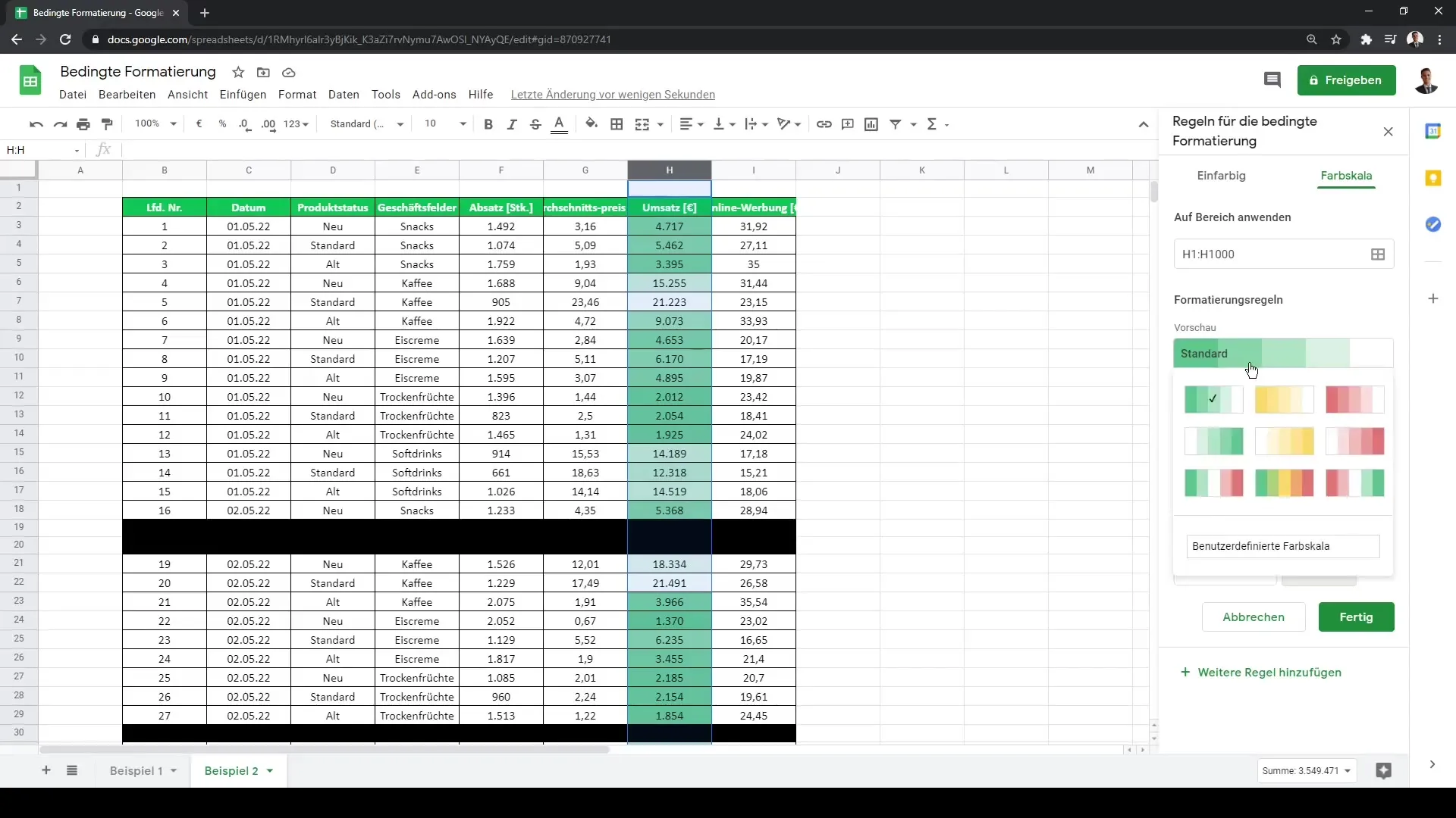
Now you have a sheet that shows at a glance what your financial data looks like and where action is needed.

Summary

In this guide, you have learned how to use conditional formatting in Google Sheets to effectively visualize your data. From color scales for displaying profits and losses to highlighting empty cells - these techniques help you interpret your data quickly and make appropriate decisions.