Google Sheets: Data analysis with the SUBTOTAL function

In this tutorial, I will show you how you can effectively use the function =SUBTOTAL in Google Sheets. With this function, you have the ability to calculate results precisely based on filtered data. Whether you need averages or sums, the SUBTOTAL function allows you to dynamically adjust your data and apply relevant calculations directly to a filtered dataset. Below you will learn step by step how to implement and apply this function.

Key Takeaways

• The function =SUBTOTAL allows for calculating subtotals for filtered data.
• You can choose different calculation methods, such as sums or averages.
• Filtering the data affects the valid results in the calculations.

Step-by-Step Guide

First, you need to prepare your data in Google Sheets. Make sure you have a dataset that needs to be analyzed.

Step 1: Filter the data

Now I will show you how to insert a filter into your data. Simply click on the filter icon in your Google Sheet. This will give you the option to filter your data based on certain criteria.

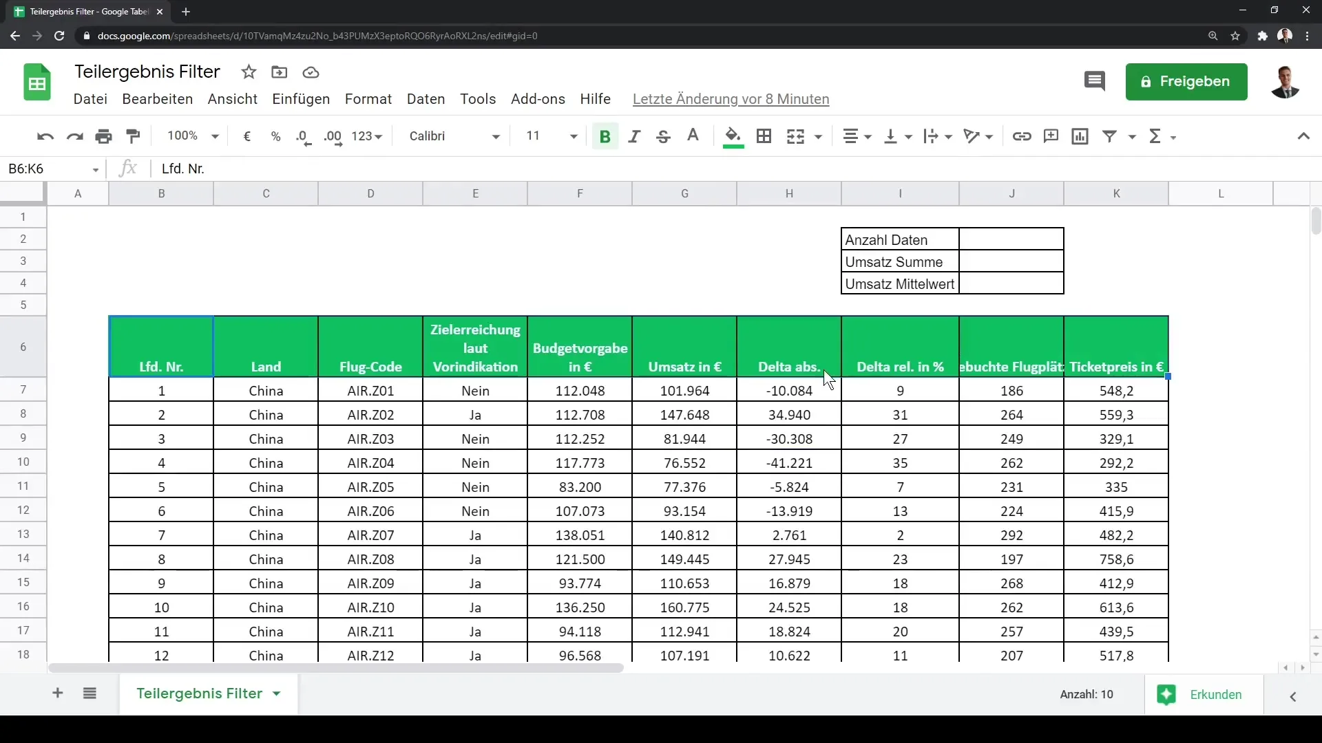
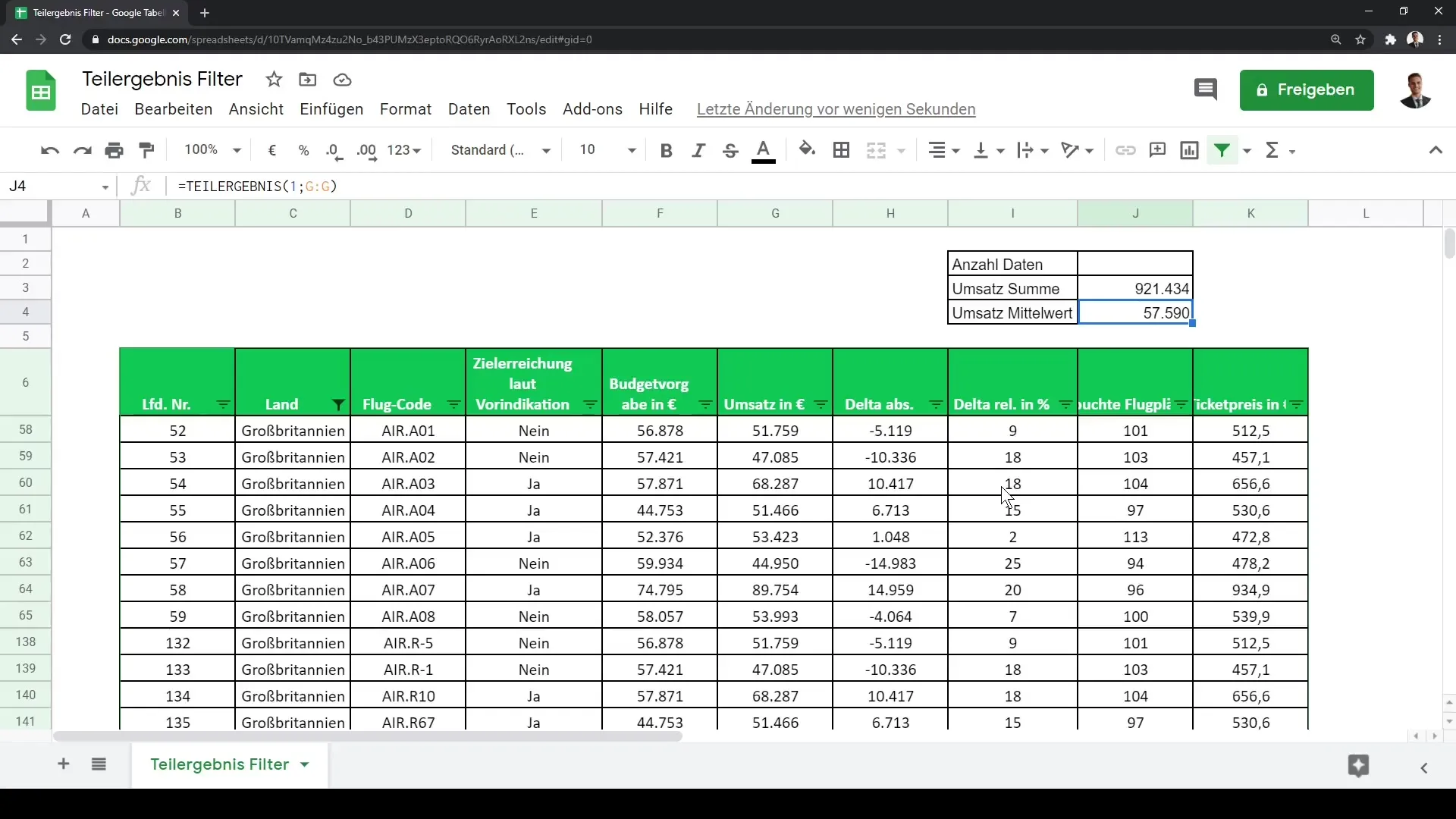
Let's say you only want to see the data for China. You can simply uncheck the other countries by removing the corresponding checkboxes. When you click "OK", only the entries for China will be displayed.

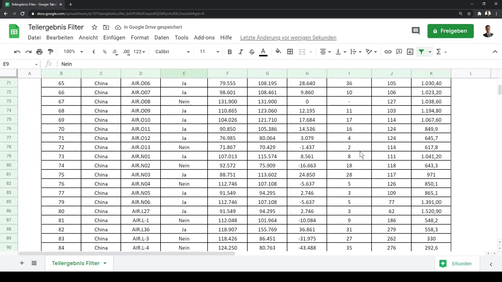
The issue here is that your existing formulas like the sum do not take into account the filtered data.

Step 2: Insert the SUBTOTAL function

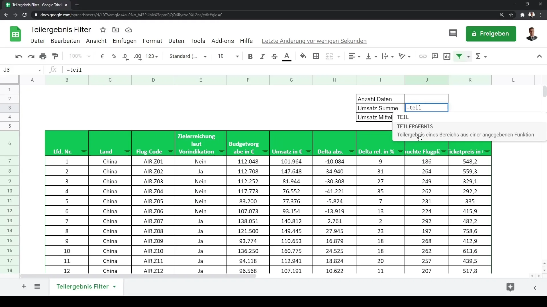
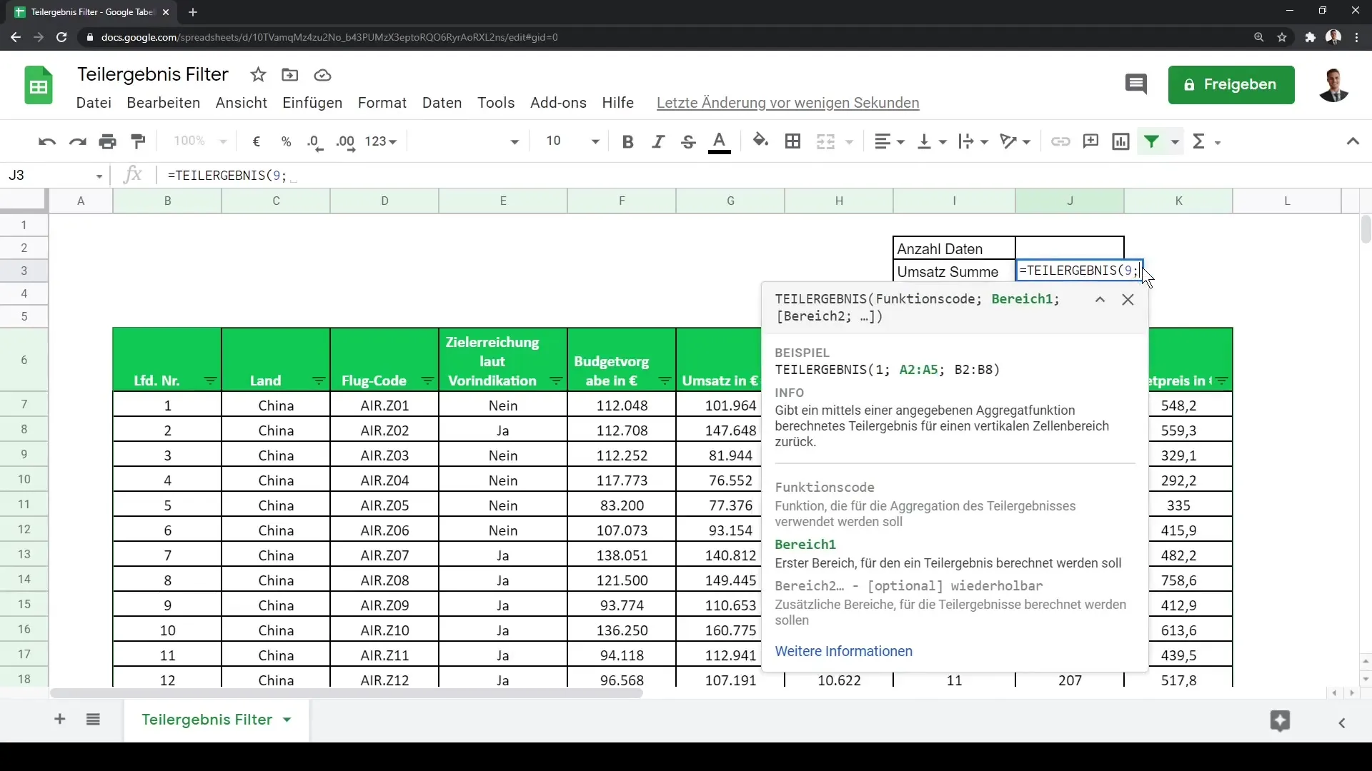
Now the advantage of the SUBTOTAL function becomes apparent. To use this function, simply enter =SUBTOTAL into a cell. This function will give you a subtotal based on a specified calculation method.

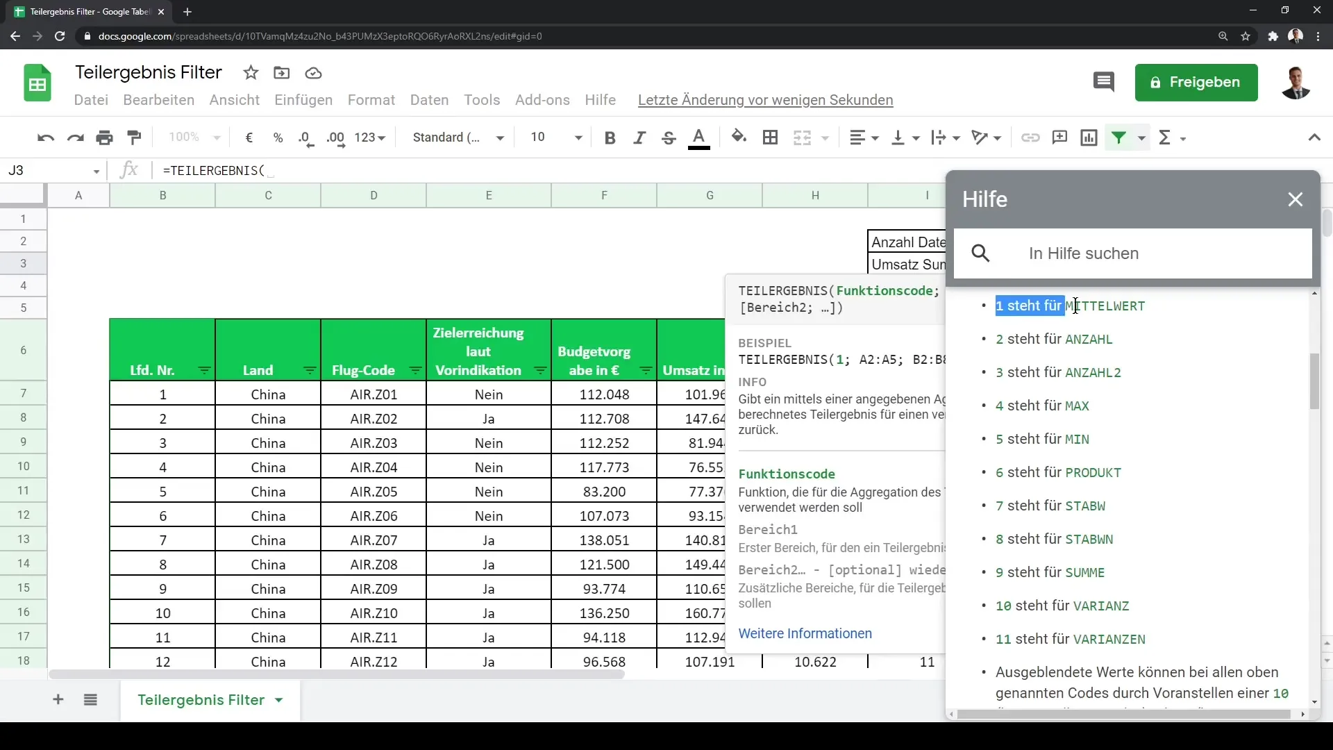
To find out which function code corresponds to your desired calculation, you can click on "more information". In this overview, you will find the various function codes. For example, 1 stands for the average and 9 stands for the sum.

Step 3: Choose calculation and define range

Assuming you opt for calculating the sum. You enter 9, followed by the cell range. You can choose your range from G7 to G1000. It is useful to choose a larger range than the actual data you have, so that adding future data is not a problem.

Now you will get the sum of all filtered data based on the criteria you have set.

Step 4: Format the results

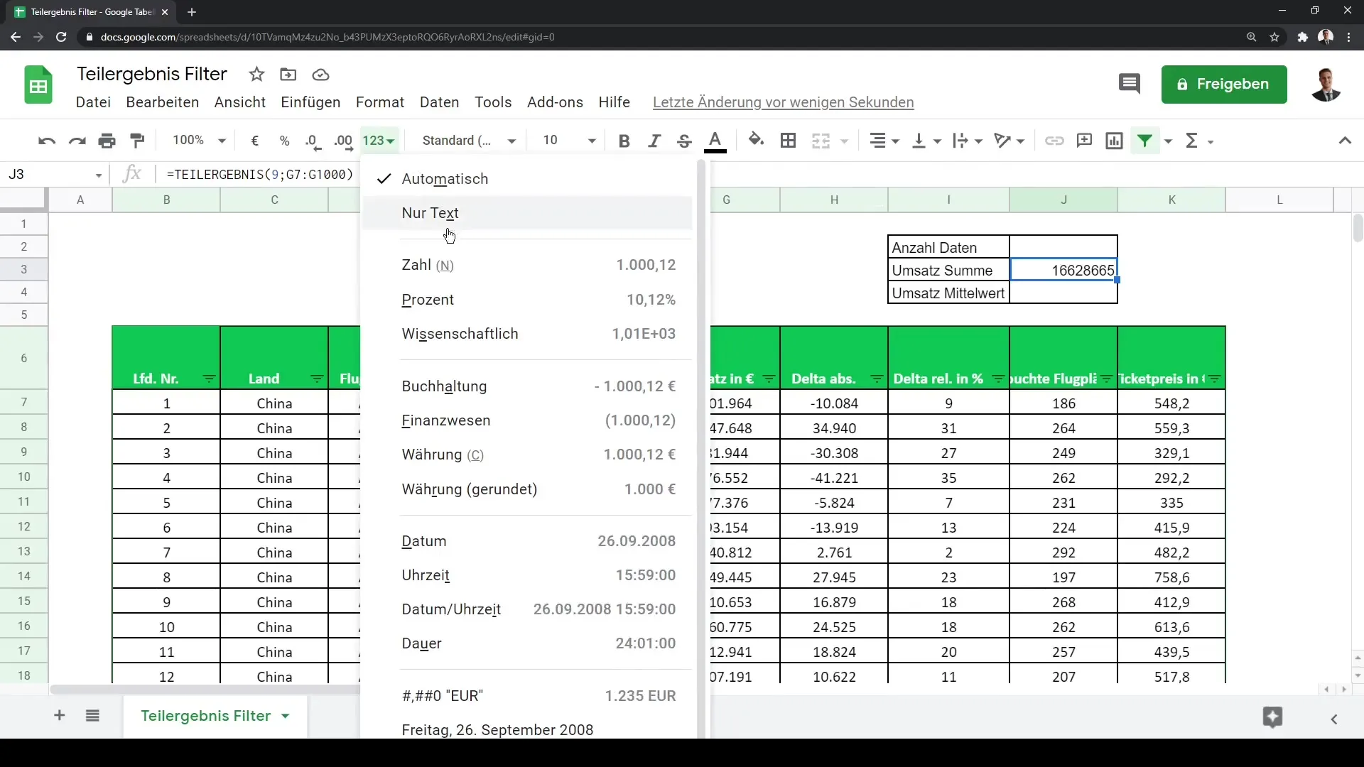
Once the sum is calculated, you can format the result, for example, as a number without decimal places.

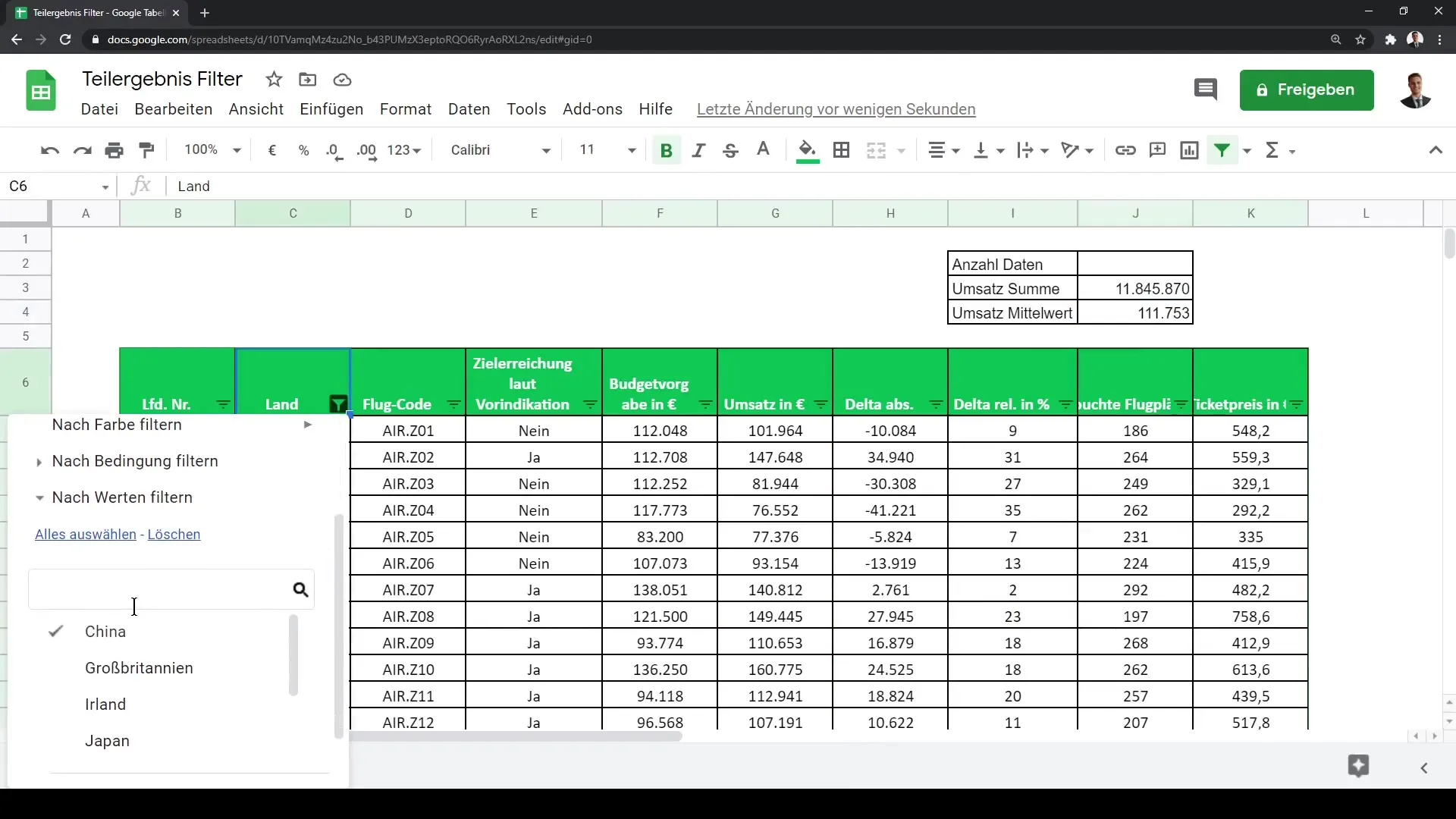
Now, when you filter the data, you will see the results adjust automatically. If you only want to select the UK, the sum for that location will be updated immediately.

Step 5: Perform further calculations

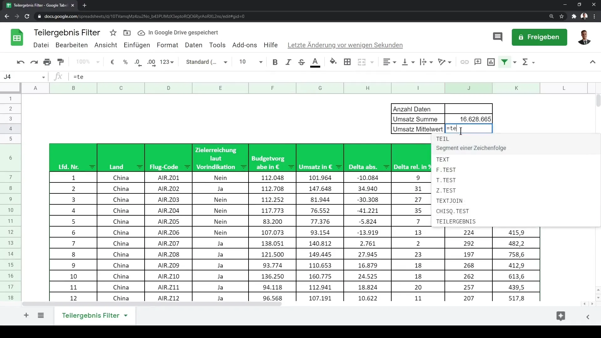
The function =SUBTOTAL can also be used for other calculations. For instance, you can perform the calculation of the average using function code 1 and select the same cell range. Again, you can display the result in the desired format.

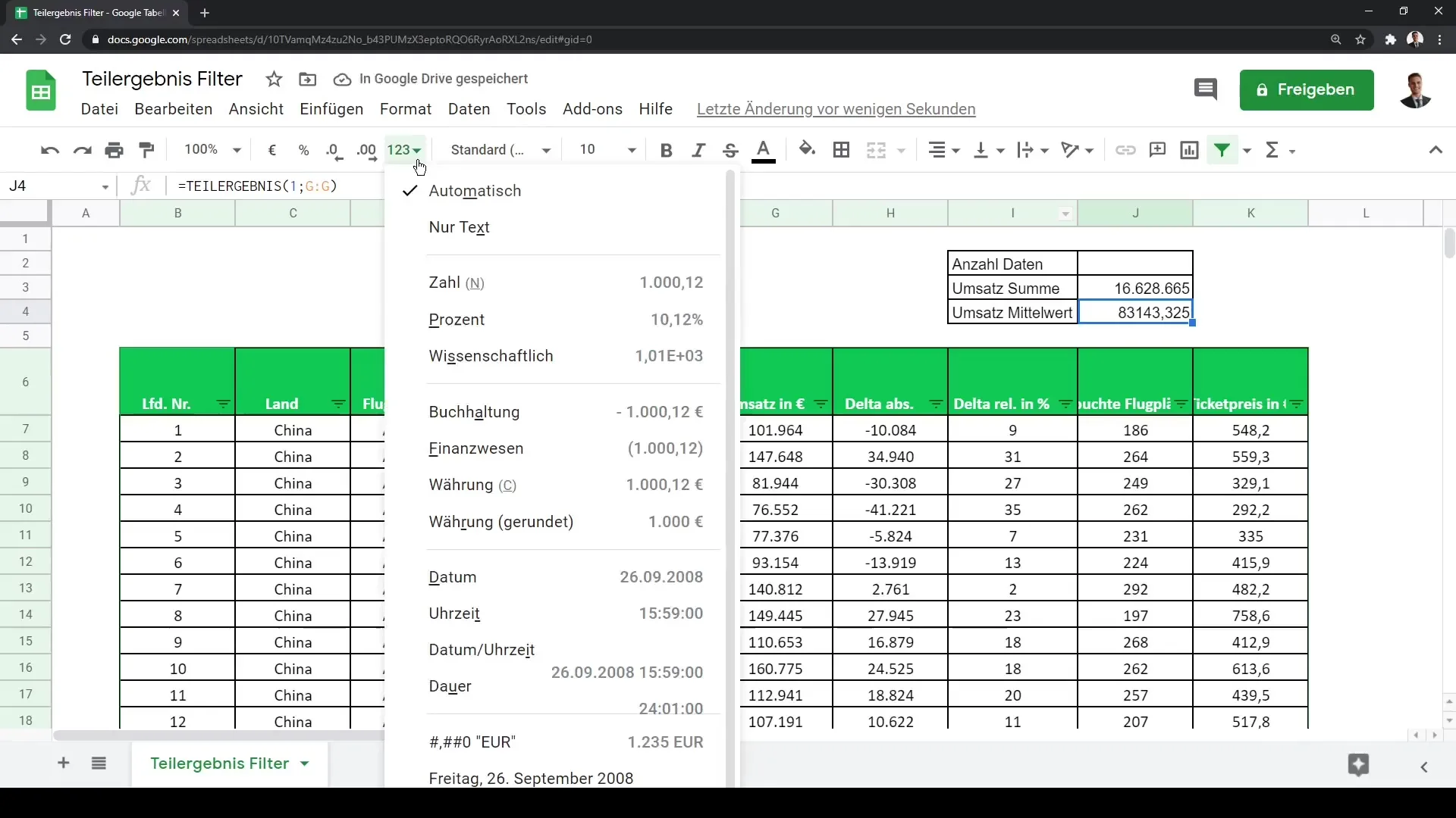
With the right filters and subtotal results, you can quickly and accurately gain insights into your data, which will update immediately when the filter results change.

Summary

In this guide, you have learned how to use the =SUBTOTAL function in Google Sheets to perform precise calculations for filtered data. You can easily filter your data and display the results in real-time for various metrics.