Data validation and dropdowns in Google Sheets

In this guide, you will learn how to use data validation in Google Sheets to create dropdown lists. Creating dropdown lists is particularly useful when you want to avoid input errors and consolidate data. Let's say you work at a university and want to uniformly record students' programs. By sensibly applying data validation, you can ensure that inputs are standardized and can be consolidated in your list.

Main Takeaways

1. Data validation helps avoid input errors and keep data consistent.
2. With dropdown lists, you can offer users a selection of predefined values.
3. You can customize data validation to reject manual inputs and display helpful input messages.

Step-by-Step Guide

Step 1: Activate Data Validation

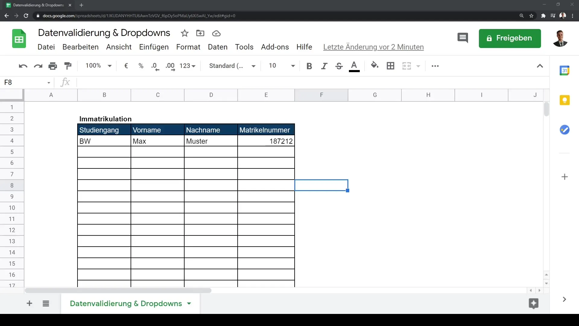
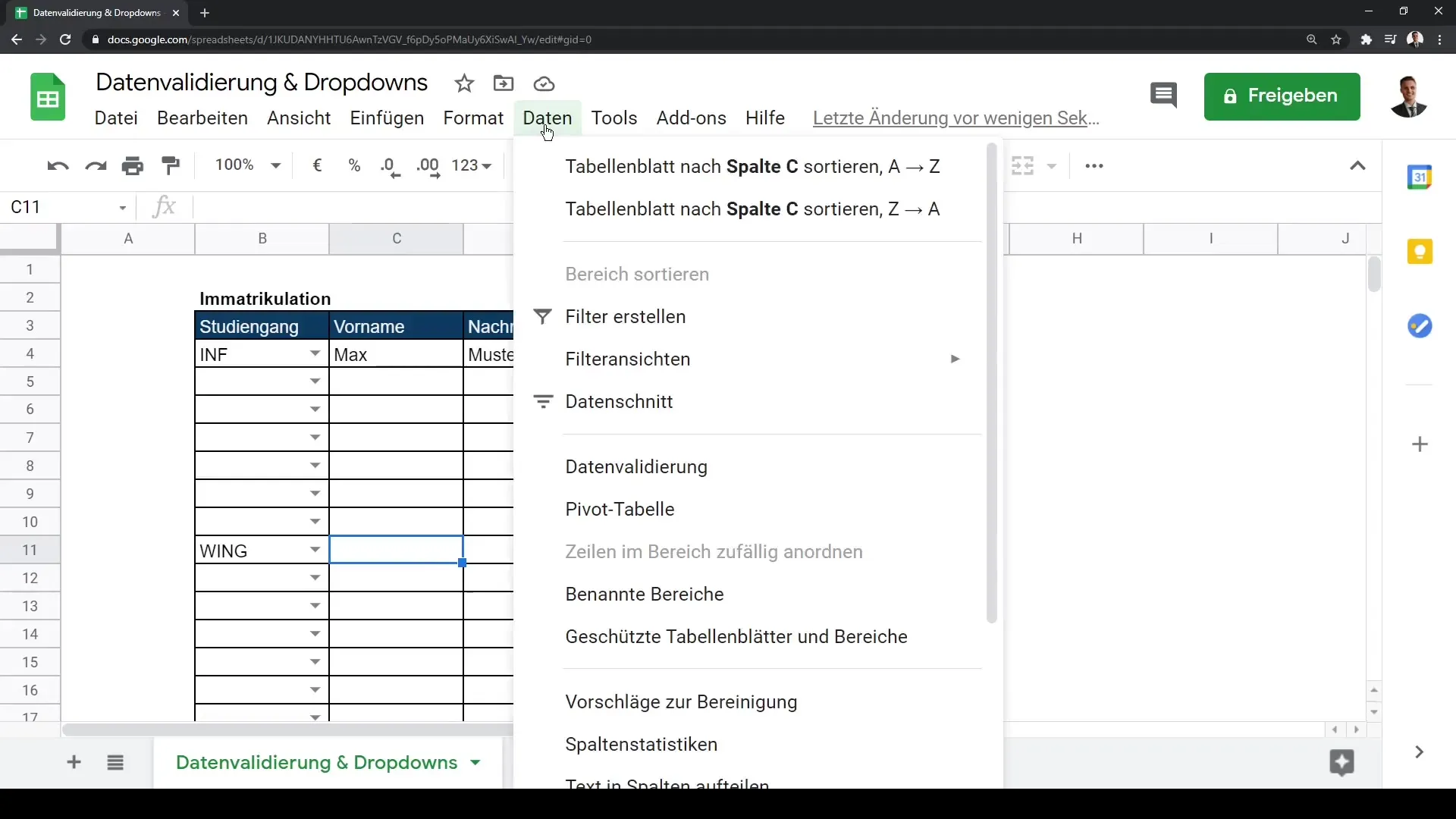
To start using data validation in Google Sheets, open your Google Sheet. Navigate to the "Data" tab and click on "Data validation." This will open a new dialog where you can make the desired settings.

Step 2: Select Cell Range

Now select the cell range you want to use for the dropdown list. For example, you could select cells from B4 to B32. Make sure you define the correct range for your data, as this is crucial for later inputs.

Step 3: Choose Criteria

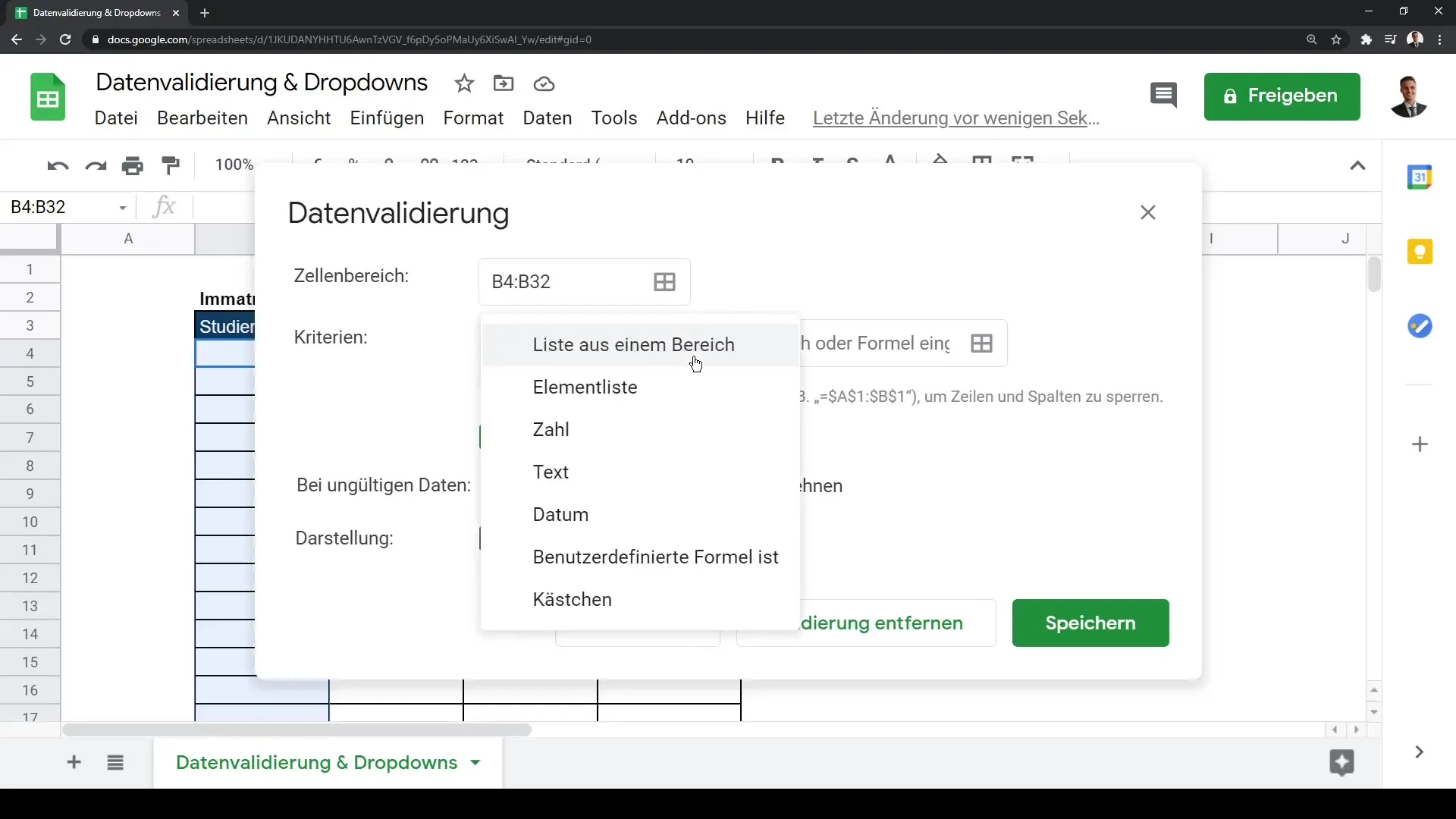
In the dialog, you can set various criteria for data validation. This means you can specify what type of inputs are allowed. You have the option to select a list or create the list yourself.

Step 4: Create Custom List

If you want to create a custom list for dropdown options, enter the desired entries. For example, you could type "BW" for Business Administration, "IF" for Business Informatics, and "CS" for Computer Science. Make sure to list all relevant programs so that students can make the right selection.

Step 5: Display Dropdown List

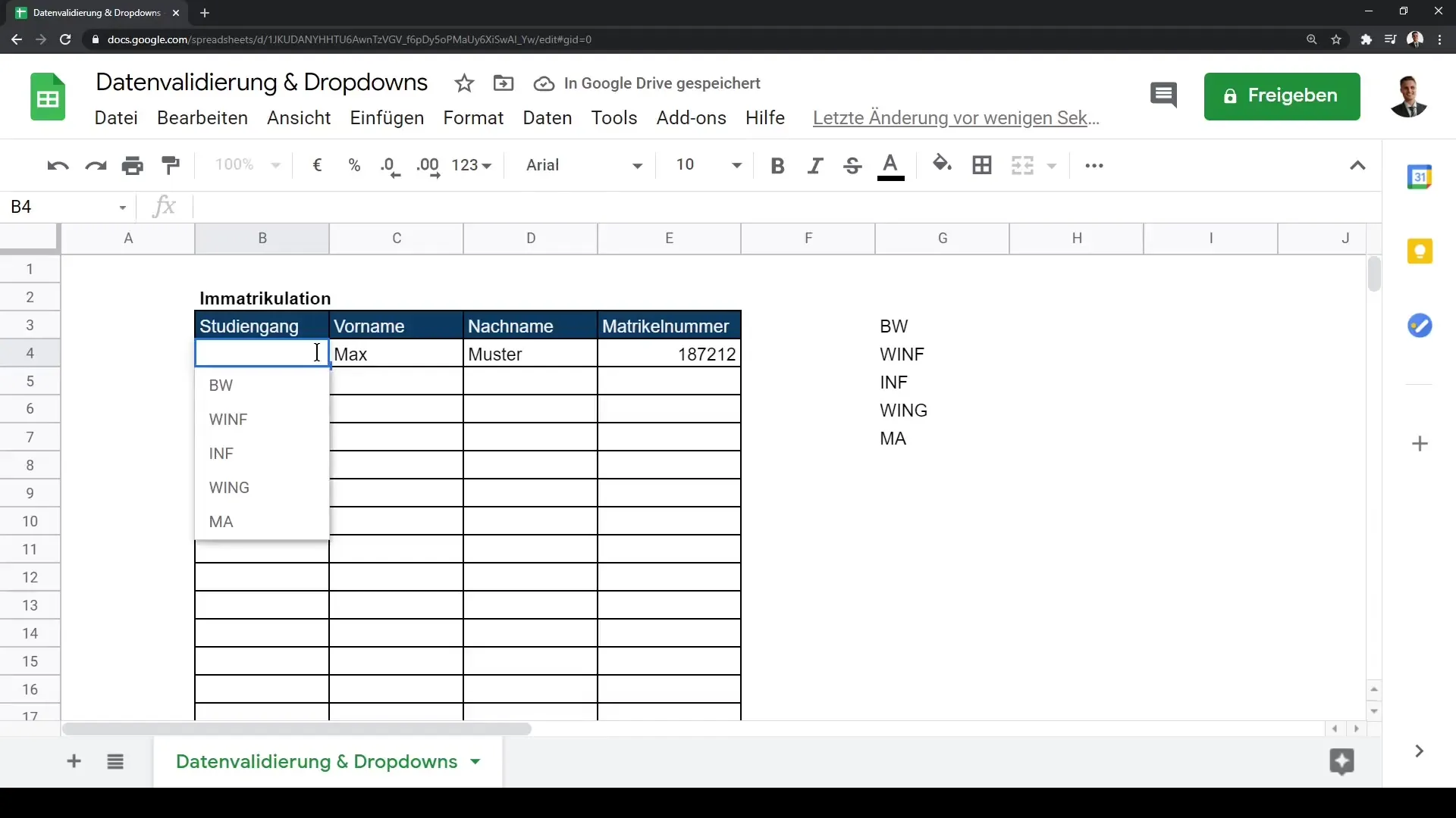
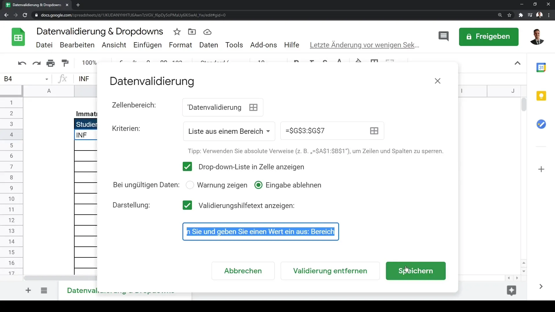
Enable the "Show dropdown list in cells" option. Then click "Save." Once the list is created, a dropdown symbol will appear in the selected cell, allowing students to choose the corresponding program.

Step 6: Reject Inputs

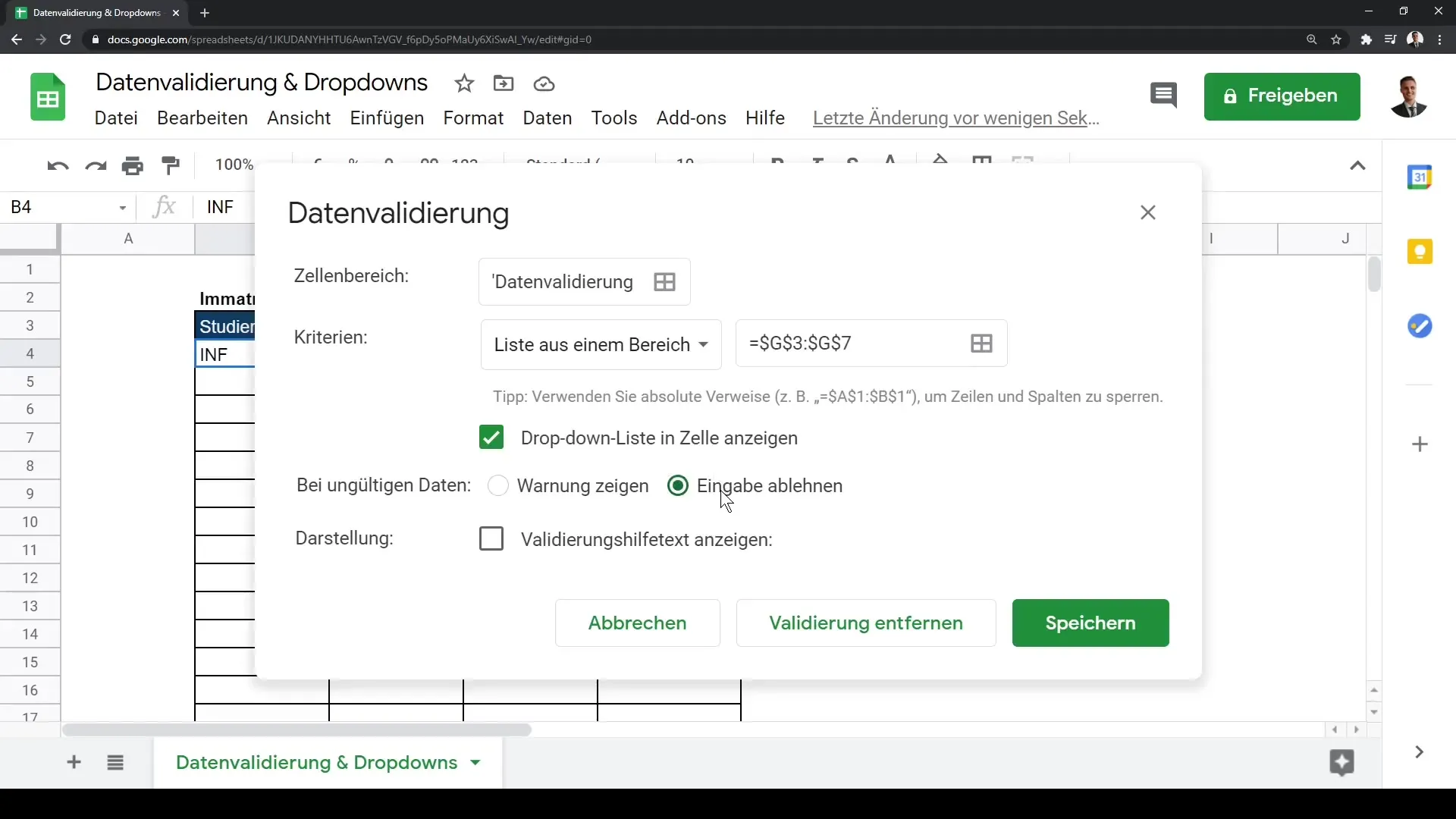
To ensure that students cannot make invalid inputs, you can reject the input. This means they cannot use self-entered values not in the dropdown list. Go back to data validation and enable the option to implement this function.

Step 7: Add Validation Help Text

An excellent way to improve user guidance is by adding validation help text. This can help inform users about what values to input. For example, you could set "Click and enter a value from the range" as help text.

Step 8: Apply Dropdowns to Additional Cells

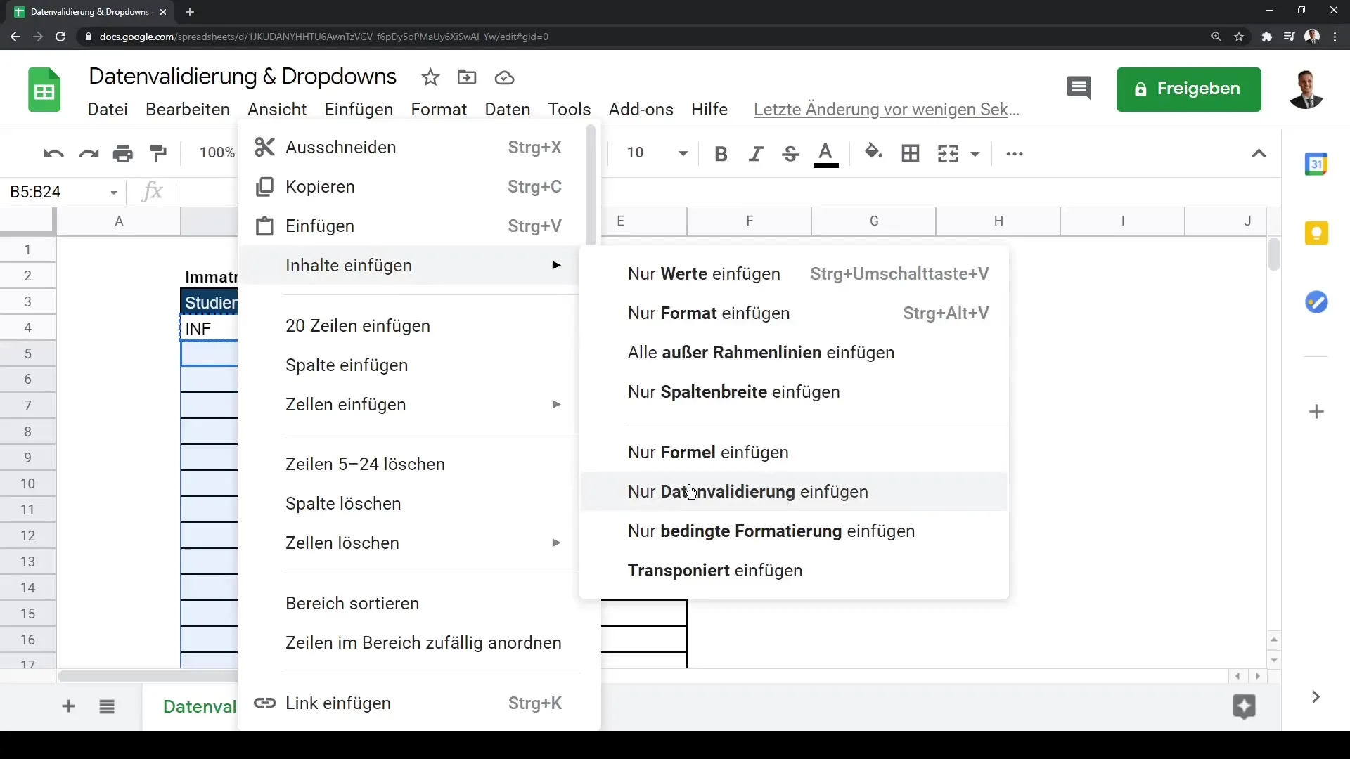
To apply the created dropdown list to other cells, you can first copy it. Use the combination "Ctrl + C" to copy the cells. Then select the target range, right-click, choose "Paste special," and then "Paste data validation only." This way, you now have the dropdown option and help text in all desired cells.

Step 9: Reviewing the Entries

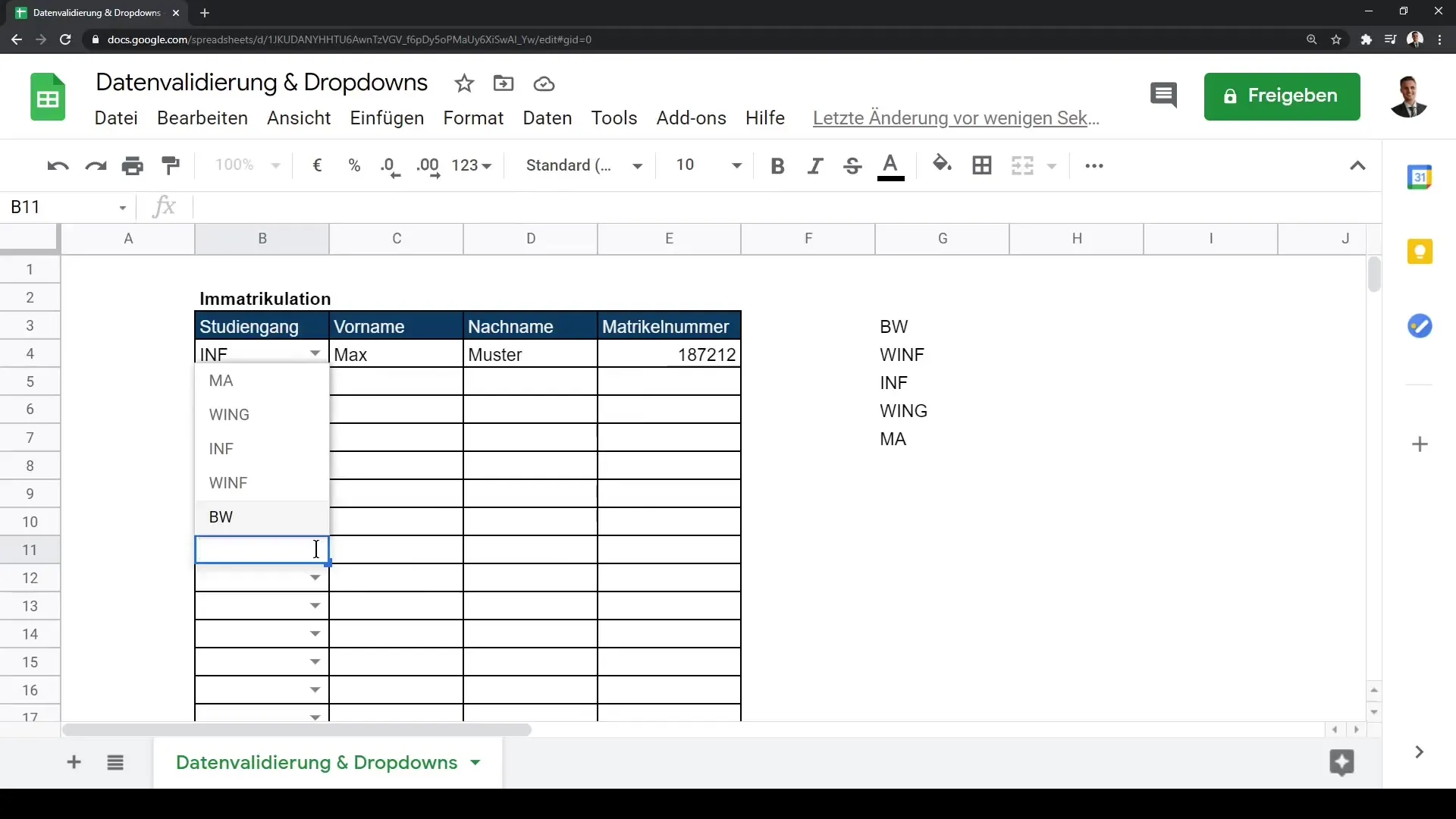
Check the different dropdown options in your Google Sheet to ensure that everything is displayed correctly. Click on the dropdown menu to see if all the created options are available and that each cell displays the prompt message.

Step 10: Conclusion and Results

You have now learned how to create dropdown lists in Google Sheets using data validation. This feature makes entering data easier and helps maintain the quality of your data records in tables. The usefulness of this technique is particularly evident when you are trying to summarize and analyze different data.

Summary

In this tutorial, you have learned step by step how to implement data validation in Google Sheets to ensure consistent and error-free data entry. You have learned how to create dropdown lists, reject entries, and enable helpful input messages.