Creating and customizing pivot tables in Excel

In this tutorial, you will learn step by step how to create and customize a Pivot Table in Excel. The lesson is based on a practice task and explains how to prepare the data, create a Pivot Table, and customize it to optimize your analysis. This process is crucial for effectively evaluating data and gaining relevant insights. Let's get started!

Key Insights

• A successful Pivot Table requires a consistent and well-structured data foundation.
• Empty cells or columns can disrupt the analysis and should be removed.
• Pivot Tables allow for effective data consolidation and presentation in various formats.
• The layout of the Pivot Table can be easily adjusted to achieve improved visual representation.

Step-by-Step Guide

Adjusting the Data Foundation

In the first step, it's about optimizing the data foundation. Here, we have a raw dataset from a hardware company focusing on the revenues of individual business areas. You will notice empty columns and cells that could disrupt the analysis.

First, you can remove the empty columns. Press Ctrl + - or right-click and select "Delete Cells." Make sure to also delete blank cells that could affect the data structure.

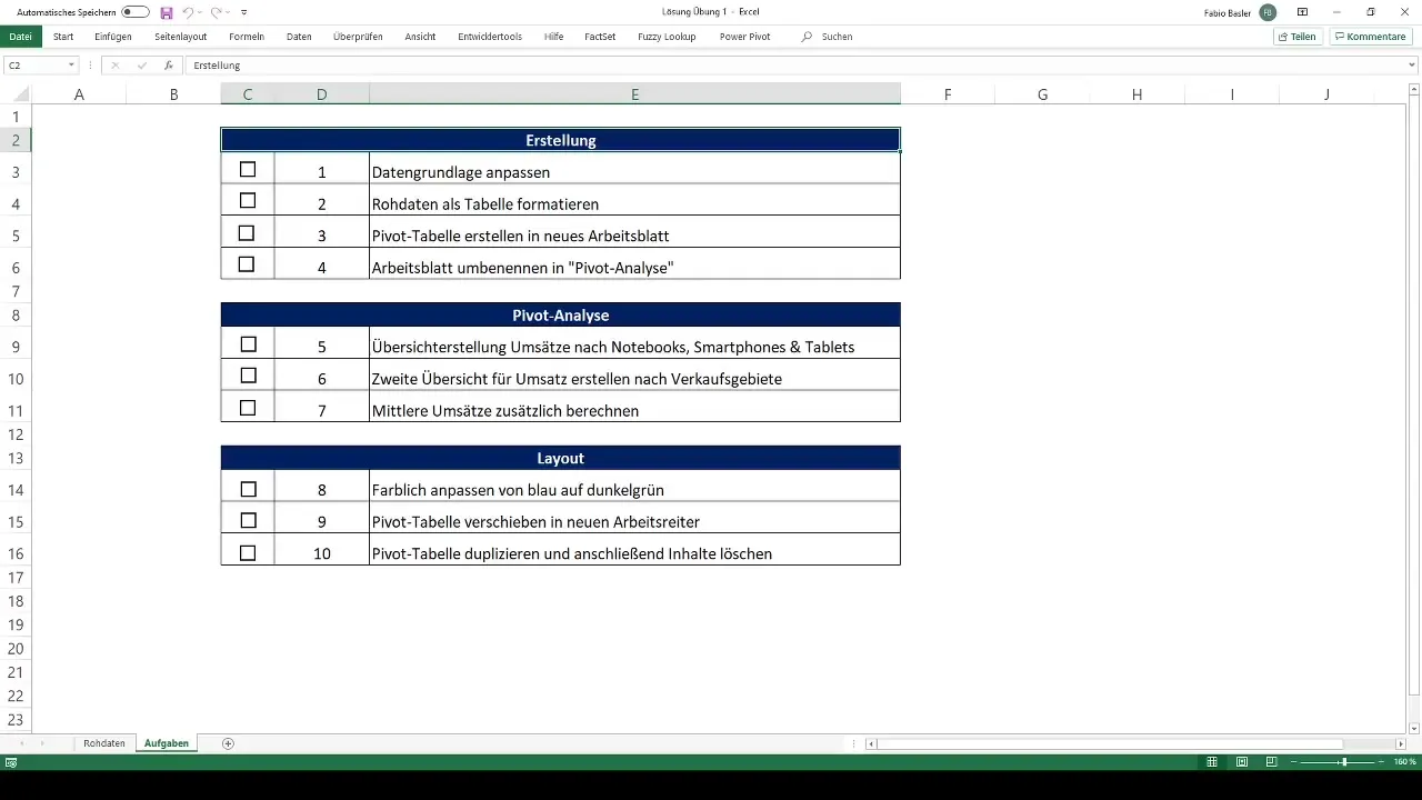
To uniformly structure the data, select the entire data range by pressing Ctrl + Shift + Down Arrow. Then, drag the selected cells to the edge of the data range to optimize the structure.

Formatting Raw Data as a Table

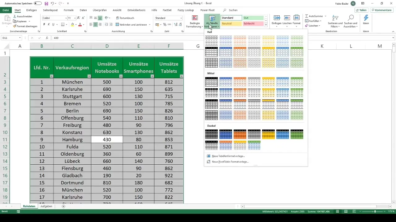
Now that the data structure is optimized, you should format the raw data as a table. Select the entire data foundation by pressing Ctrl + A again. Then press Ctrl + T or go to "Format as Table."

Choose an appropriate formatting, such as the light blue one. Make sure to include the headers. Once you do this, the formatting will be visible in the table tools.

Creating the Pivot Table

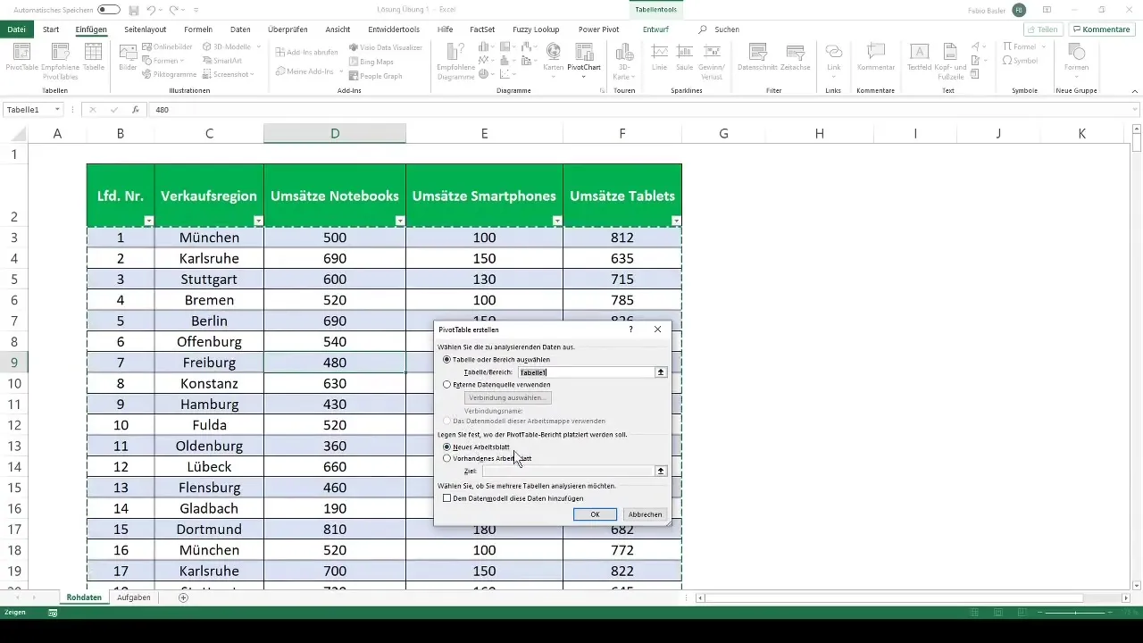
Now it's time to create the Pivot Table. Click anywhere in the table to make the table tools and the option "PivotTable" visible. Alternatively, you can also go to the "Insert" tab and select "PivotTable." The entire table will be automatically selected, and you can create the Pivot Table on a new worksheet.

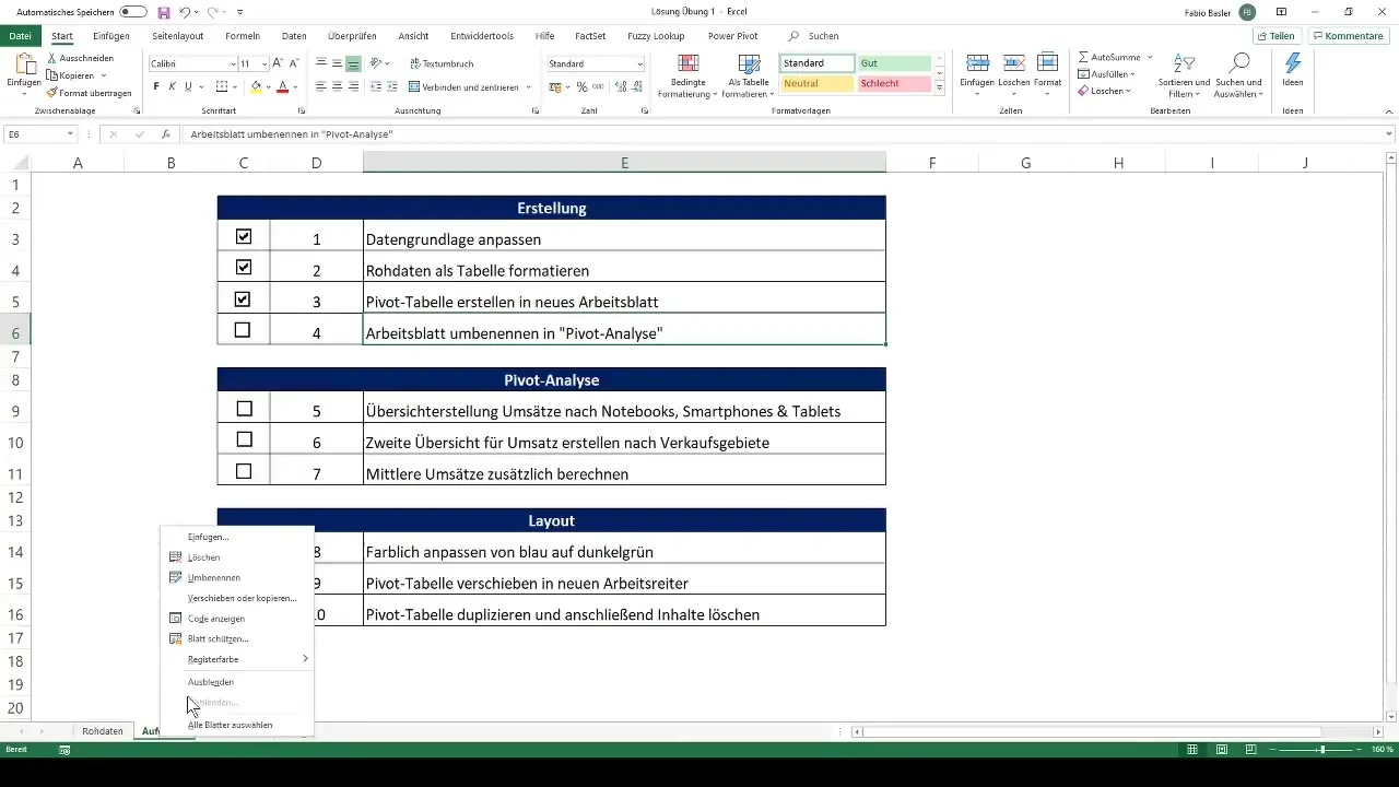
Now you already have the empty Pivot Table. To make it more organized, rename the worksheet by right-clicking on the tab and selecting "Rename." Name the sheet "Pivot Analysis" and color it to highlight the tab.

Analyzing Revenues by Categories

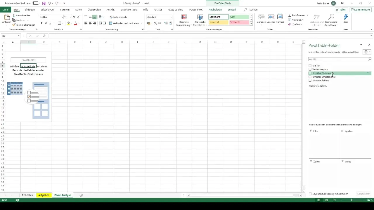
Now you want to create an overview of revenues by categories. Click into the Pivot Table. On the right side, you should see the Pivot Table fields. Drag the revenues for Notebooks, Smartphones, and Tablets into the Values area.

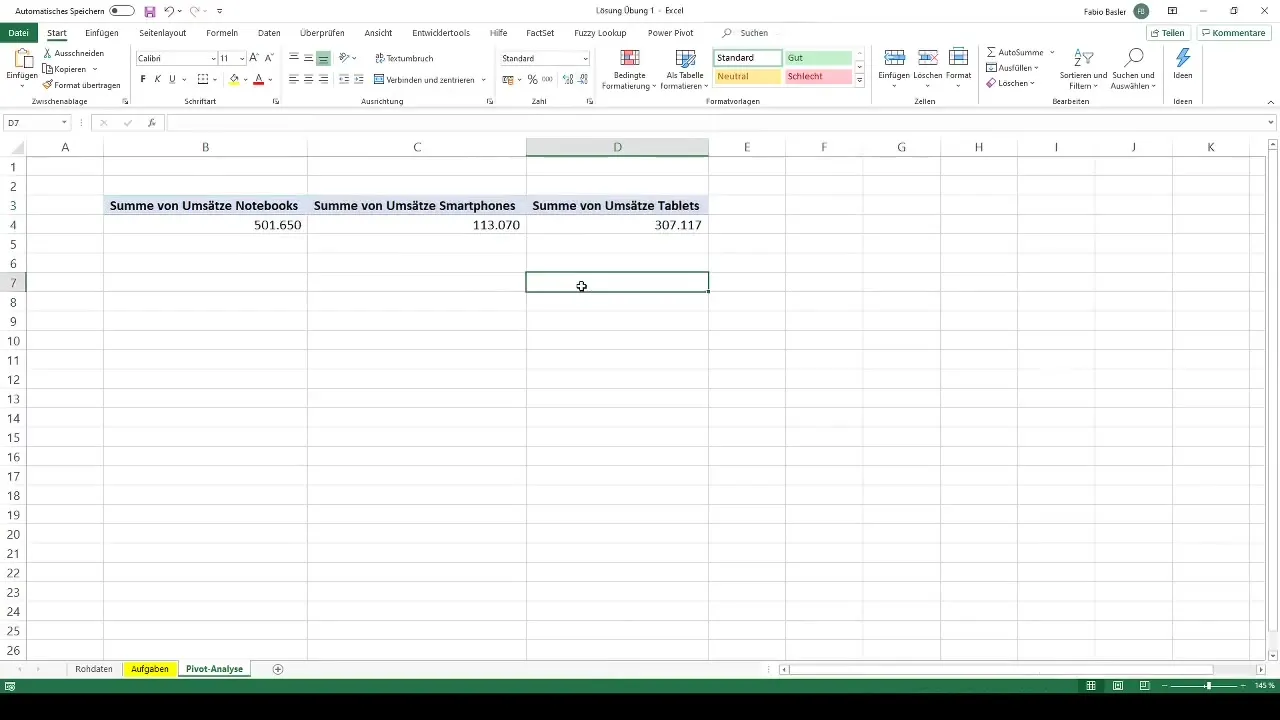
You can add another row to view the consolidated total revenues. Format the results by adding the thousand separator and removing decimal places. Now you should see clear revenue numbers.

Creating Second Overview

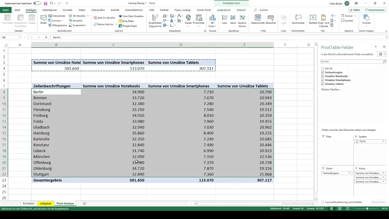
In the next step, we will create a second overview of revenues broken down by sales cities. Click back into the Pivot Table. To create the second overview, you can either create a new Pivot Table or copy the existing one (Ctrl + C) and then paste it (Ctrl + V) into a different area.

Additionally, drag the sales regions into the row fields of the Pivot Table to get the desired breakdown.

Calculating Average Revenues

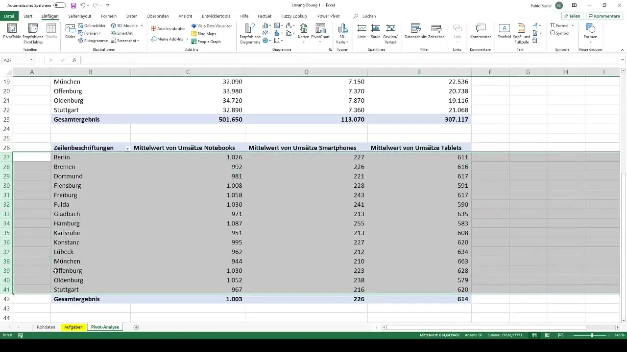
Now it's time to calculate the average revenues. You can continue to use the second pivot table. Copy it again. Click on the values and select "Value Field Settings" to change the summary to "Average." You will now see the average revenues broken down by business areas and sales regions.

Customizing the Layout of Pivot Tables

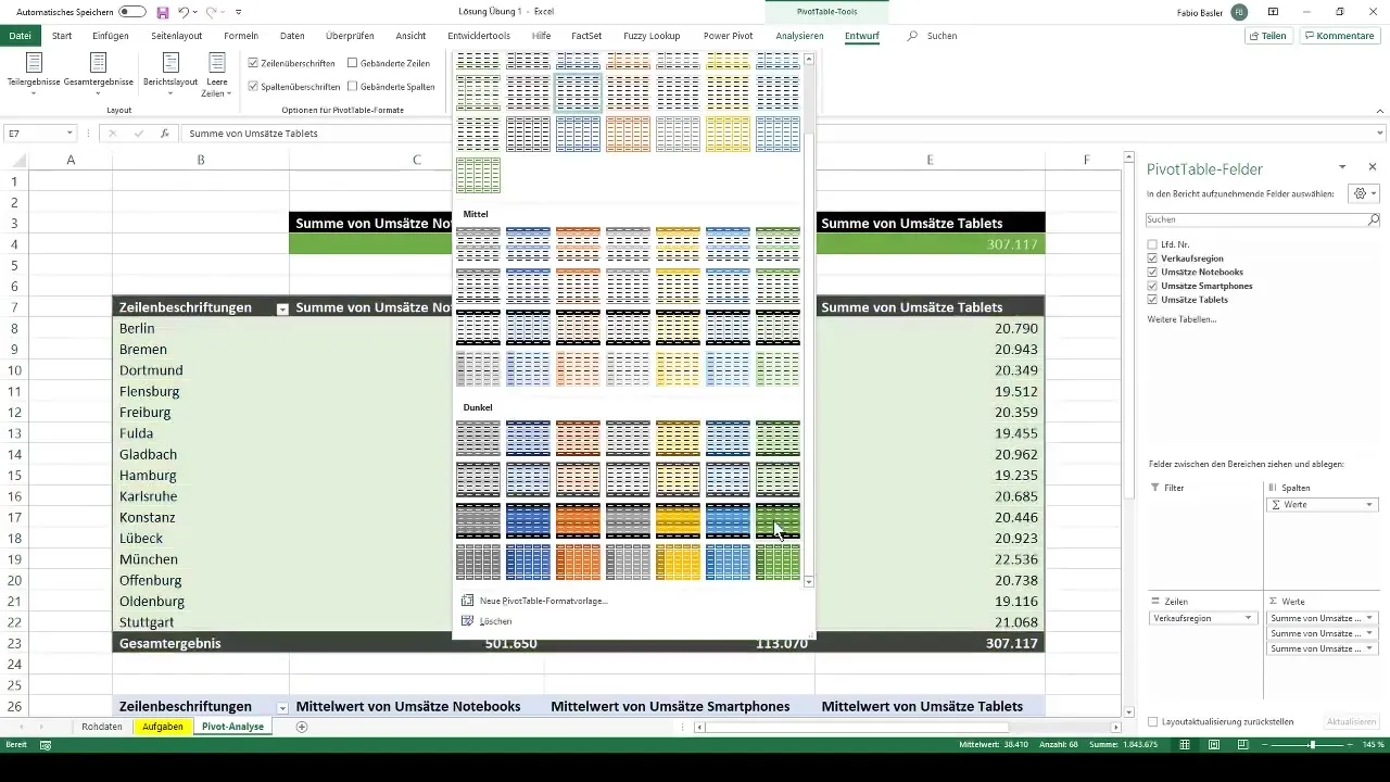
In the final step, you want to visually enhance the layout of your pivot tables. Switch to a pivot table and go to the Pivot Table Tools. Choose the Design and adjust the colors to appear dark green. This will ensure a consistent and visually appealing presentation of your data.

Moving Pivot Table to New Worksheet

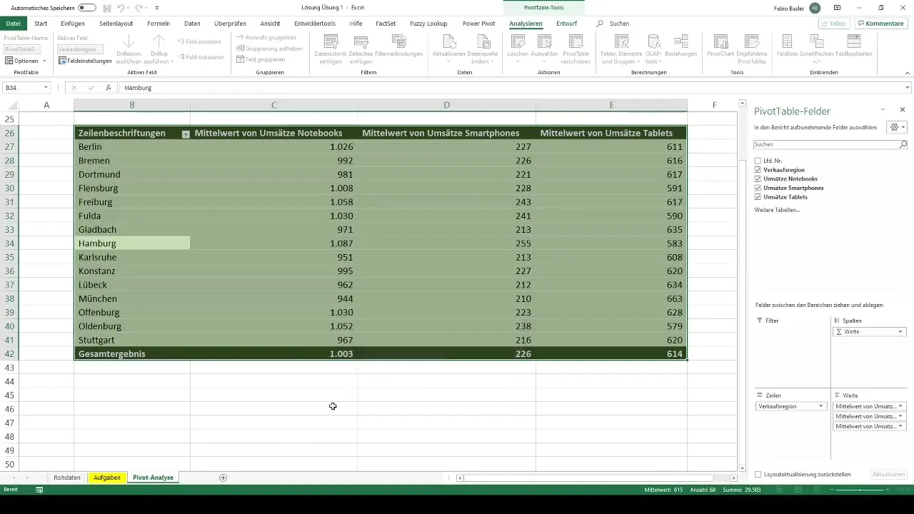
To optimize the last pivot table for space, you need to move it to a new worksheet. Highlight the entire pivot table, go to "PivotTable" and choose "Move." Rename the new worksheet accordingly.

Duplicating and Clearing Pivot Table Contents

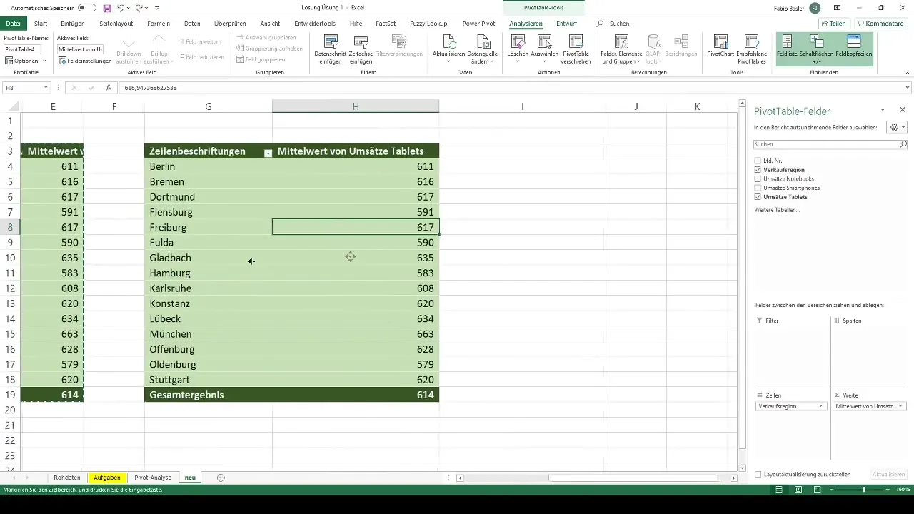
Finally, after making all the adjustments, you want to copy the pivot table and clear the contents. Highlight the entire table, copy it, and paste it where desired. Finally, delete all contents so that an empty pivot table remains.

Summary

You have now successfully mastered all 10 tasks. By following the steps presented, you will be able to effectively create and customize your own pivot tables. Take the time to experiment with the various features Excel offers. Now proceed to the next section, which deals with the different visualization possibilities of pivot tables.