Sorting and filtering pivot tables in Excel

In this guide, you will learn how to effectively sort and filter pivot tables in Excel. We are using a data set from the pharmaceutical industry with various active ingredients and their corresponding key figures. Sorting and filtering this data can help you gain better insights into your evaluations. These steps are essential to make the data more clear and meaningful.

Main Insights

• Pivot tables allow for easy sorting and filtering of data.
• You can sort the data by various key figures such as research expenses and success rate.
• Using data filters and slicers provides a user-friendly visual representation of your analyses.

Step-by-Step Guide

Step 1: Creating a Pivot Table

To sort and filter your data, start by converting your existing data into a pivot table.

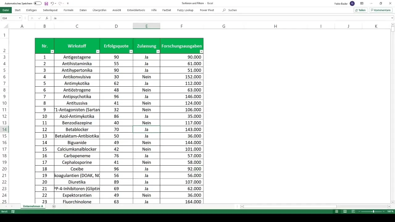
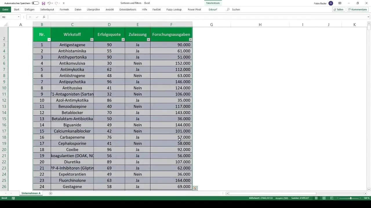
First, select all relevant data and press the shortcut "Ctrl + T" to format the data as a table. Then go to the "Insert" tab and select "PivotTable" to create the pivot table in a new worksheet.

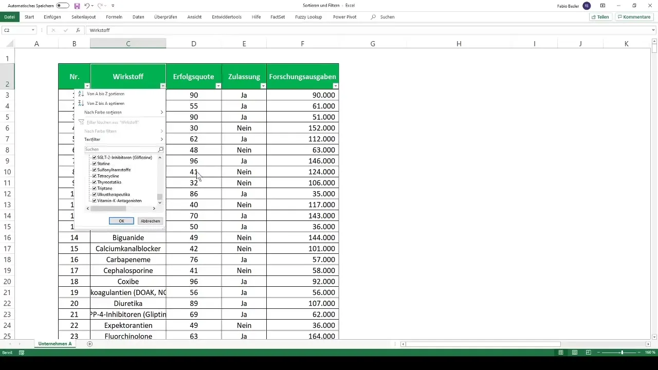
Step 2: Customizing the Pivot Table

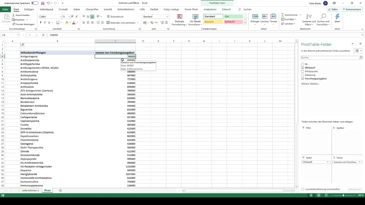
Once the pivot table is created, you can customize it by adding the desired key figures.

In our case, we add research expenses by active ingredients to better analyze the expenses. You can also add other key figures such as success rate to enable a more comprehensive analysis.

Step 3: Sorting the Data

Now, let's get to the actual sorting of the data. You want to sort the research expenses in ascending or descending order.

To do this, go to the menu bar and click on "Data". Then select the "Sort" option. You have the option to sort by different criteria such as ascending or descending. Choose ascending sorting, for example.

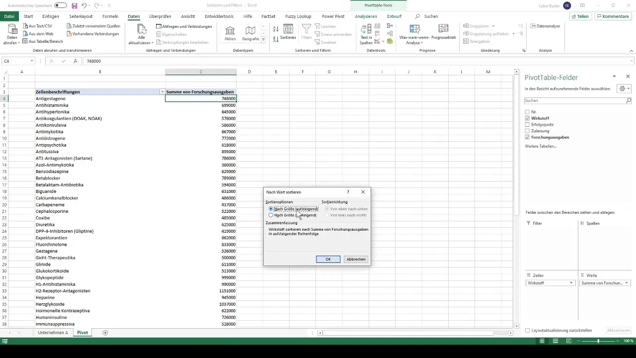
Step 4: Sorting Alternatives

If you want to sort the data by specific letters, such as A to Z or Z to A, you can also use these options.

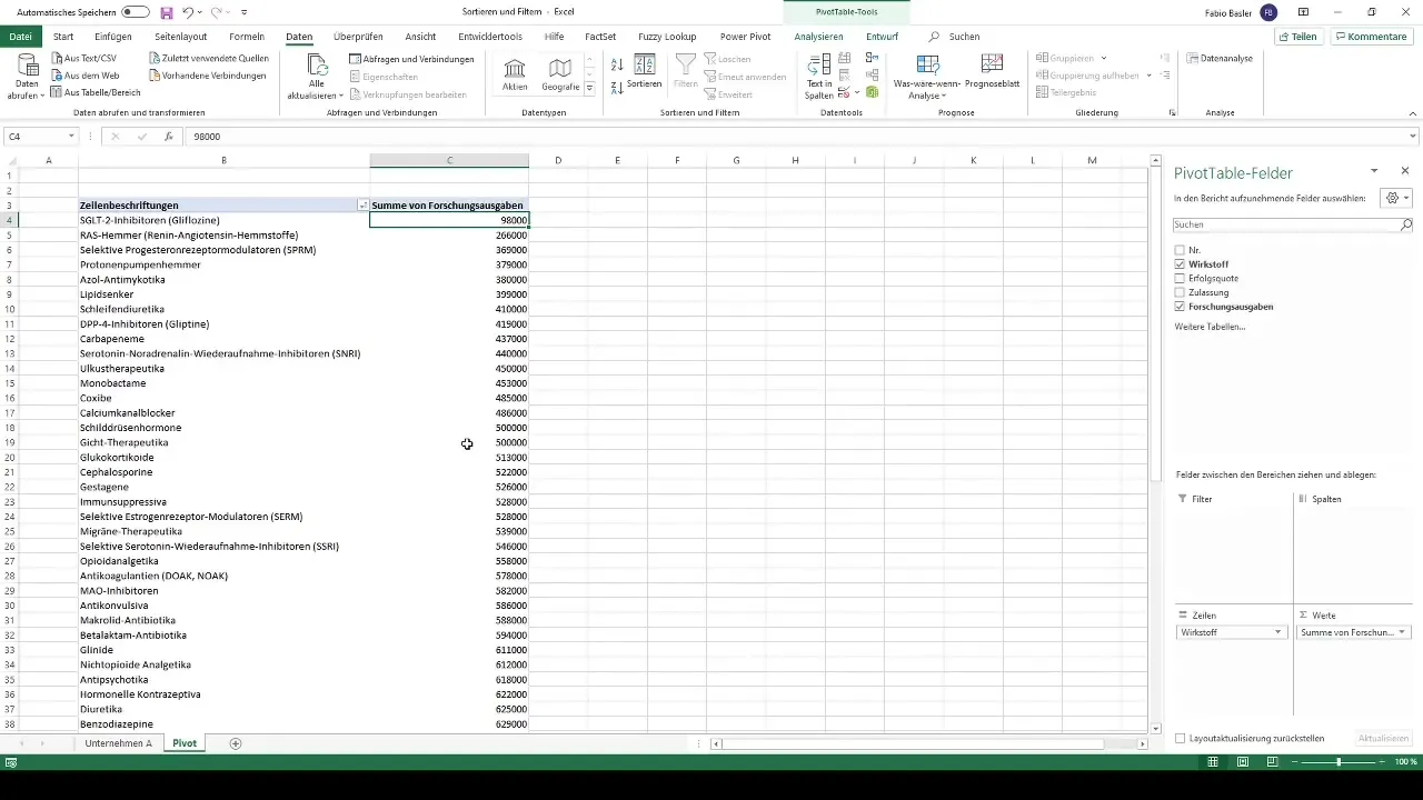
This sorting can be applied not only to values but also to the entire column or the entire raw data set of the pivot table.

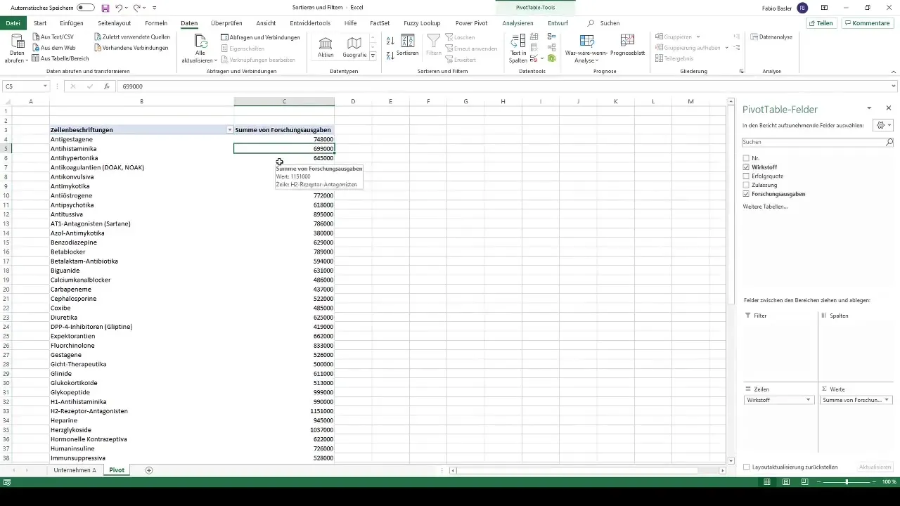
Step 5: Conditional Formatting

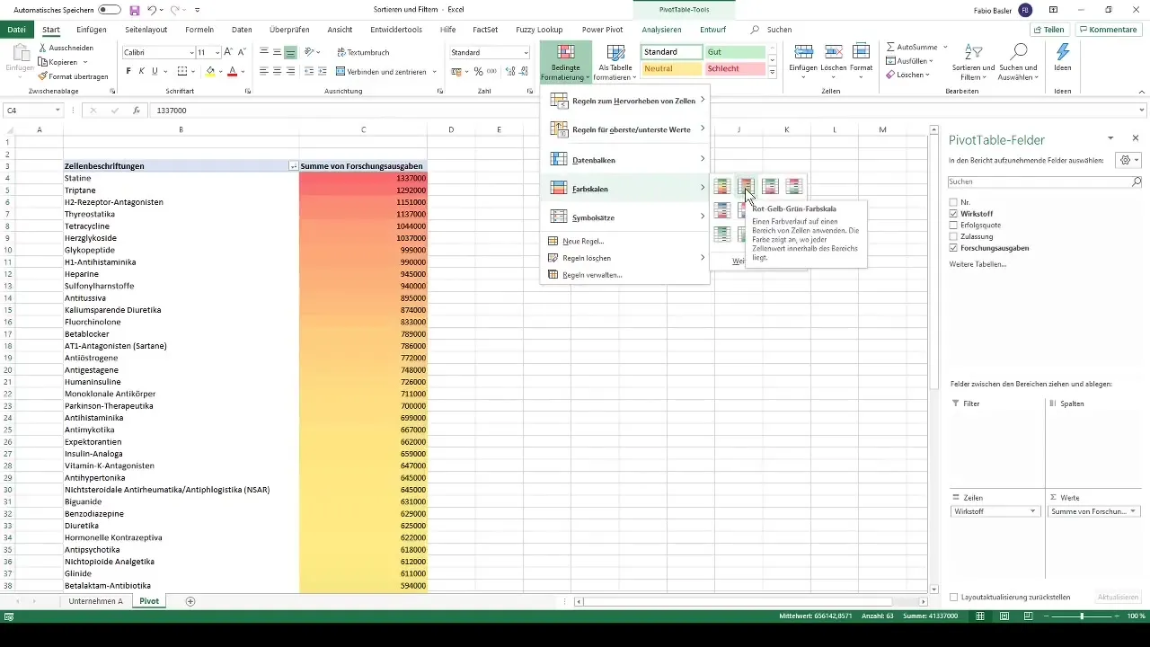
To increase clarity, you can also apply conditional formatting. This helps you visually represent the values.

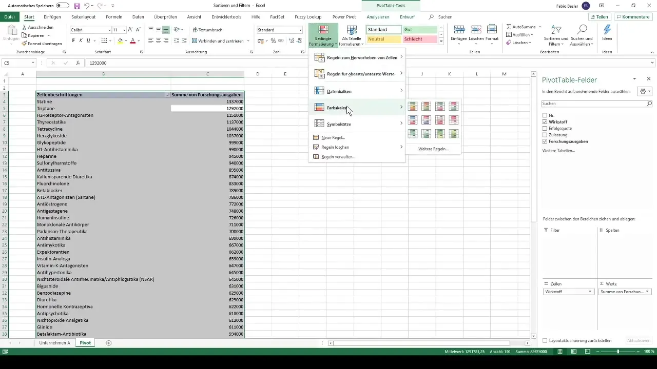
Go to "Conditional Formatting" and choose a color scale, e.g., red-yellow-green, to highlight the highest and lowest values.

Step 6: Adding the Success Rate

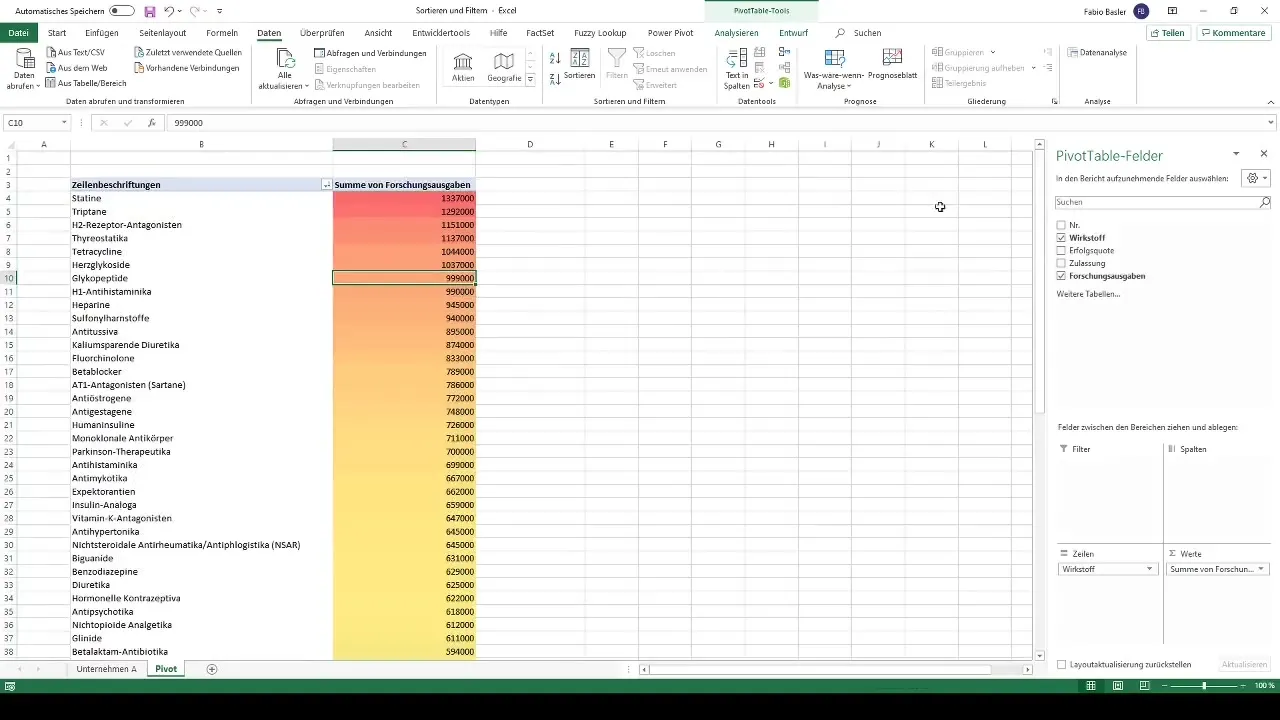
After visually formatting the research expenses, you can add the success rate as a second key figure. In this step, you should calculate the average to correctly represent the success rate.

Step 7: Filtering the Data

Next, you can filter the data according to specific criteria. For example, you may only want to see the approved active substances.

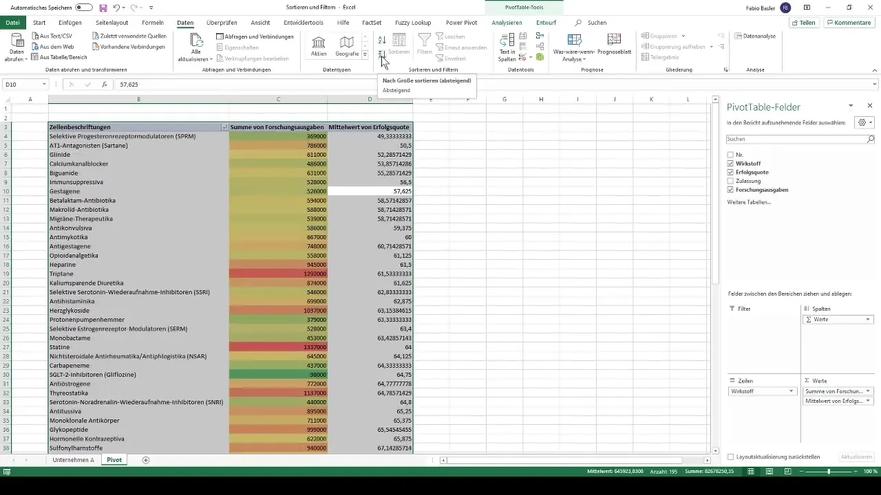
Drag the approval column into the filter area to filter the data accordingly and display only the relevant entries.

Step 8: Using Slicers

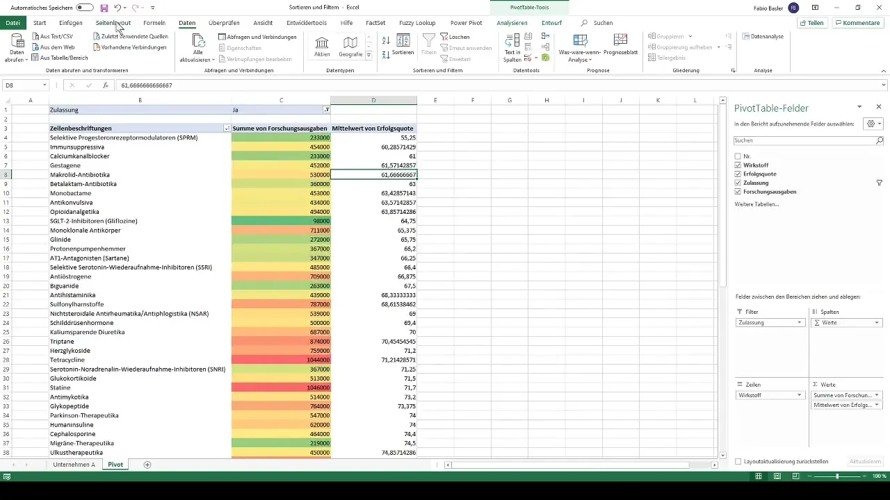
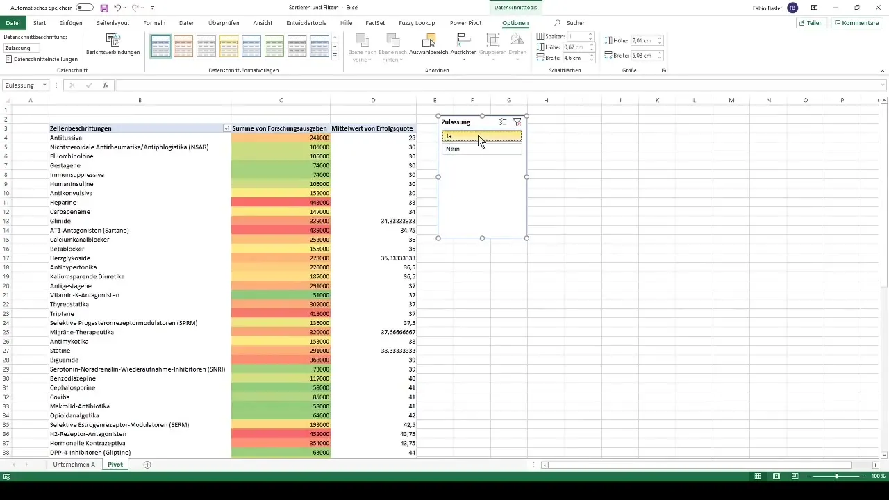
Another way to visually filter the data is by using slicers. You can add a slicer for approval to toggle between approved and unapproved active substances.

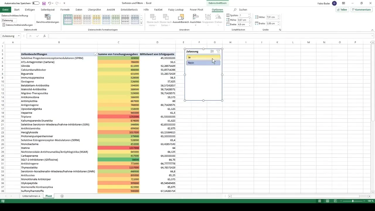
The slicer provides a user-friendly way to interactively edit the pivot table.

Summary

In this tutorial, you learned how to sort and filter pivot tables in Excel. From creating the pivot table to sorting the data to using interactive slicers, you were able to learn various techniques to present your data more clearly and gain valuable insights.