In this guide, you will learn how to calculate complex key figures using Pivot Tables in Excel. Specifically, the focus is on creating new fields from existing fields and applying various analysis methods. Understanding such advanced functions is not only helpful for data analysis but also for presenting and interpreting data in reports and presentations. Let's dive right into the topic!
Main Insights
- You can calculate new key figures with calculated fields in Pivot Tables.
- It is possible to apply different calculation methods to your data.
- Pivot Tables offer a flexible way to analyze and present large datasets.
Step-by-Step Guide
1. Understand the Basics
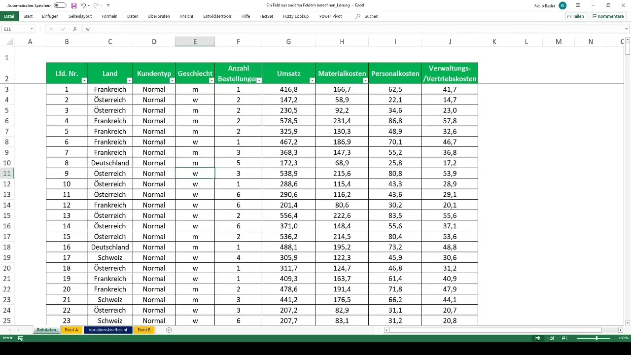
First and foremost, you should ensure that you are familiar with the dataset you want to analyze. You have a dataset that includes sales figures, material costs, personnel costs, and administrative costs. These data points are crucial because you will base your calculations on them. It is important that you understand the structure and content of the data before starting the analysis.
2. Create a Pivot Table
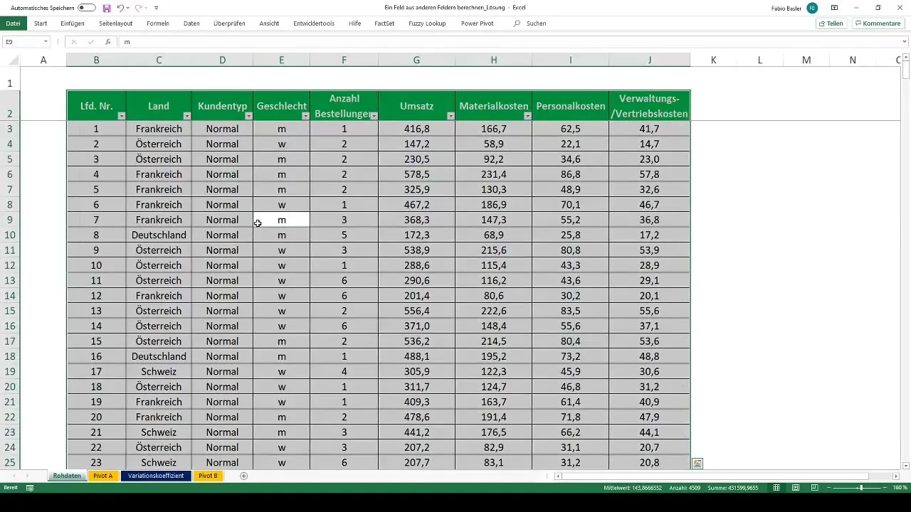
To create a Pivot Table, first select your entire dataset, including headings. Then go to Insert and select PivotTable. This allows you to bring the data into an easily understandable analysis form. Make sure to choose the correct option so that the table is created in a new worksheet.
3. Arrange Data in the Pivot Table
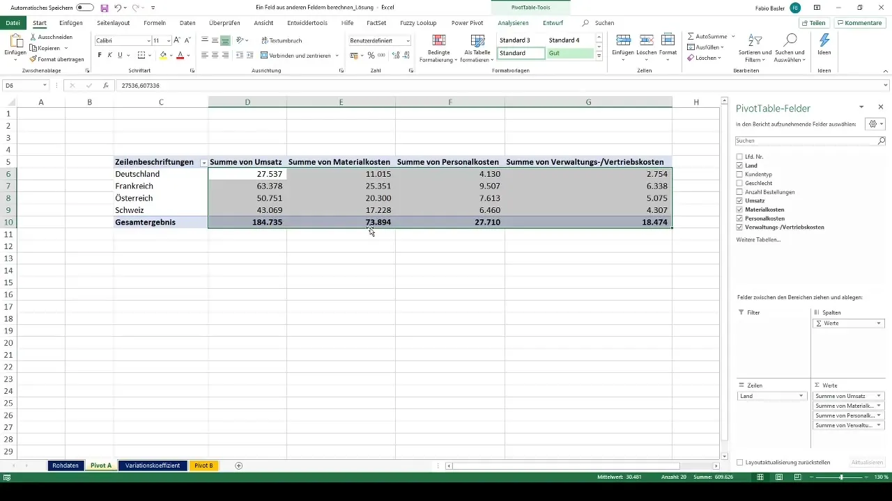
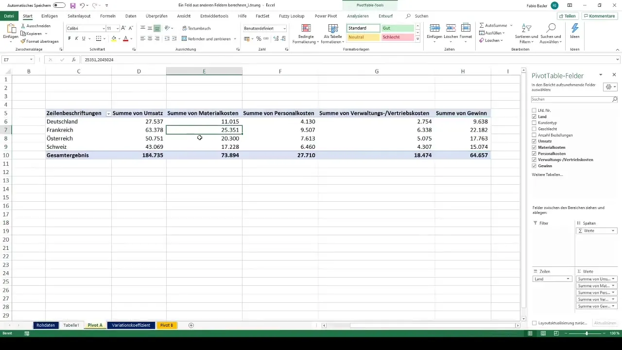
Now it's time to arrange your data in the Pivot Table. Drag the fields for sales, material costs, personnel costs, as well as administrative and sales costs into the values area of the Pivot Table. You can also drag the country field into the rows area to segment the analysis by countries. This will help you better understand the financial metrics and identify larger patterns in the dataset.
4. Format the Values
Once the Pivot Table is created, you can format the values in an appealing way. Go to the value field settings option to add a thousand separator and adjust decimals as needed. A clean and appealing presentation of your data makes a big difference.
5. Add Calculated Fields
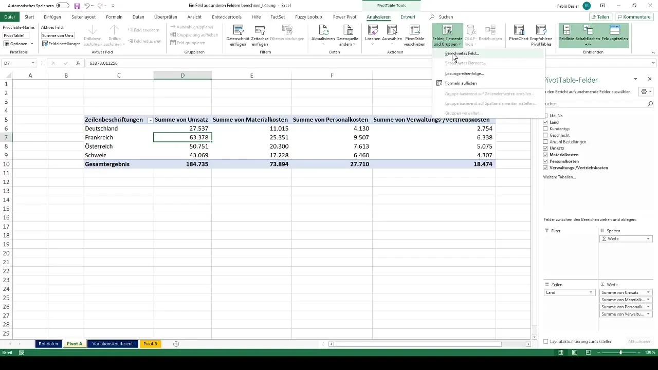
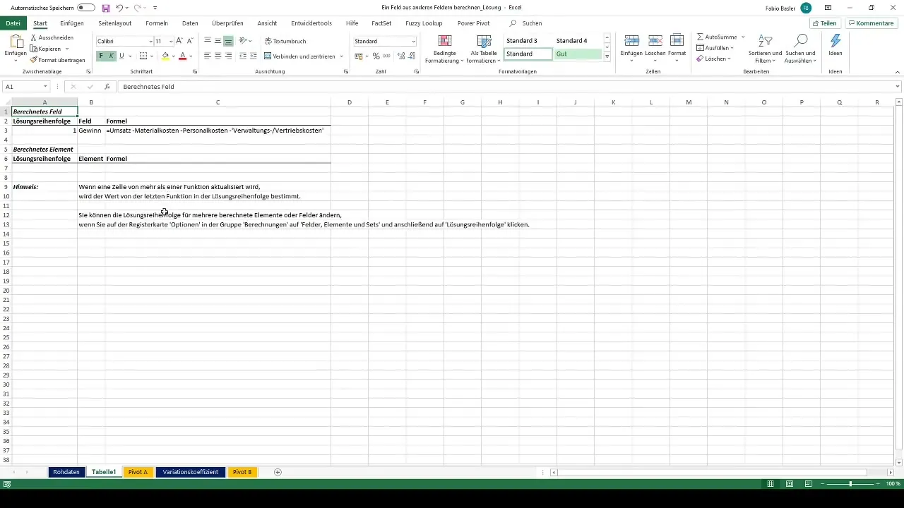
Now comes the exciting part: the calculated fields. To create a new key figure, such as profit, you can't just use the standard functions. Effectively, you take the sales field and subtract the cost categories (material, personnel, and administrative and sales costs). This is done simply using the calculated field function. After entering the formula, confirm with OK. Your profit will now be displayed in the Pivot Table.
6. Verify the Calculations
You can always check if your calculations are correct by listing the formula or analyzing the underlying calculation methodologies. Using the analyze function, you can ensure that everything is set up correctly. Make sure that the profit is actually represented as sales minus costs.
7. Customize the Calculation Methods
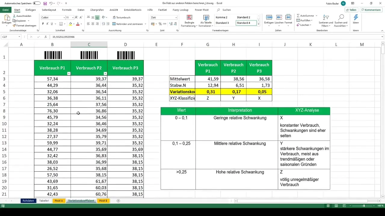
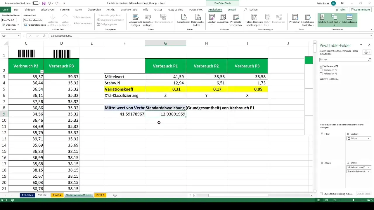
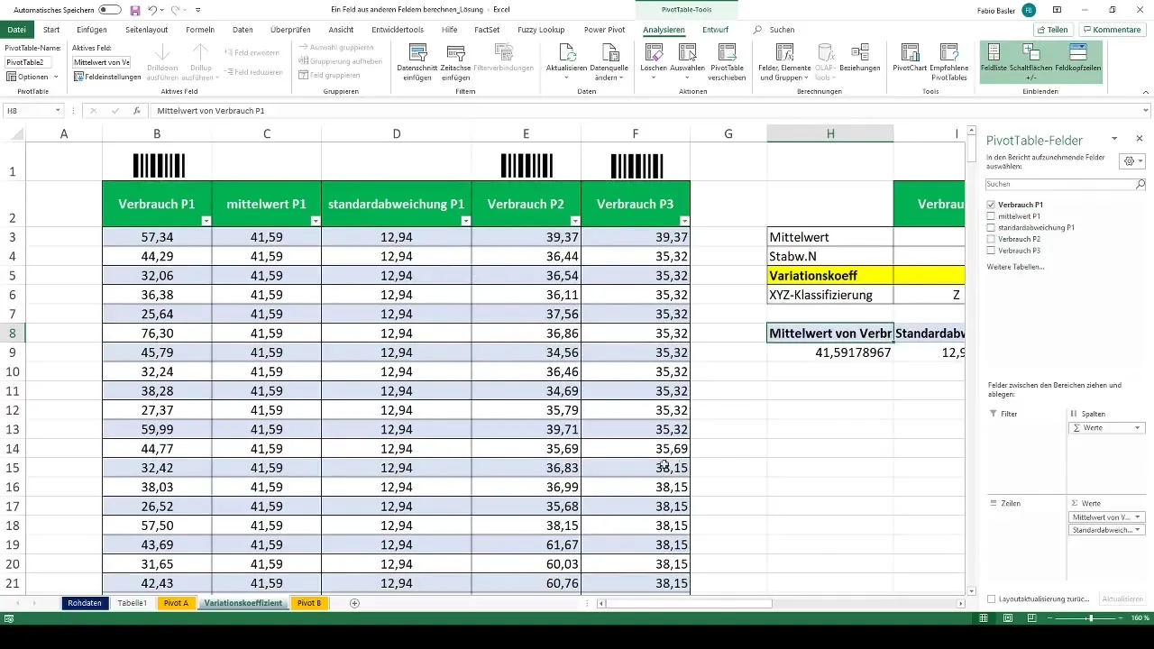
The flexibility of Pivot Tables means that you can also create other key figures. You have the option to calculate the average or standard deviation of costs or revenues. Once again, use the menu for calculated fields and adjust the calculations as needed.
8. Conduct Advanced Analyses
Another point to consider is calculating the coefficient of variation. This metric measures the relative dispersion of the data and provides you with information on the consistency of your revenues or costs. To calculate this, once again use a calculated field and type in the formula for the coefficient of variation (standard deviation divided by the mean).
9. Automation and Data Update
Once you have created your pivot table, it is easily updateable. If the underlying data changes, you just need to update the pivot table to incorporate the new data into the calculation. This is done through the refresh function, which is part of the options.
10. Conclusion and Next Steps
Now that you have the basics of creating and editing pivot tables and calculating from existing fields, you can apply this knowledge in further projects. Actively approach your data and experiment with different metrics to further enhance your analytical skills.
Summary
In this tutorial, you have learned how to work with pivot tables in Excel. You have been guided through the steps of data analysis, from creating the pivot table to using calculated fields to generate new metrics such as profit and coefficient of variation. You have understood the importance of correctly formatting and verifying data. Use this knowledge in your future data analyses!
Frequently Asked Questions
How do I add a calculated field in a pivot table?You go to the calculated fields option in the pivot table menu and enter the desired formula.
Can I use multiple calculated fields in a pivot table?Yes, you can add as many calculated fields as you want to determine different metrics.
What should I do if the pivot table does not display the correct data?Check your data source and make sure all necessary fields are included in the pivot table. Also, refresh the table to ensure you are seeing the latest data.
How often should I update the pivot table?It is recommended to regularly update the pivot table, especially when the underlying data changes.
Can I print or export pivot tables?Yes, you can print pivot tables or export them as an Excel file or PDF.


