Create and format pivot tables in Excel

In this guide, you will learn step by step how to create and format a Pivot Table in Excel. Pivot tables are a powerful tool for analyzing and summarizing data. They allow you to structure and visualize large amounts of data in an intuitive way. Whether you want to break down sales by regions or compare the performance of different business units, pivot tables help you evaluate the information quickly and efficiently.

Main Insights

To successfully create and format a pivot table, you must first format your raw data as a table. Then you can create the pivot table, drag the desired data into the correct structure, and ultimately adjust the presentation to obtain a clear analysis.

Step-by-Step Guide

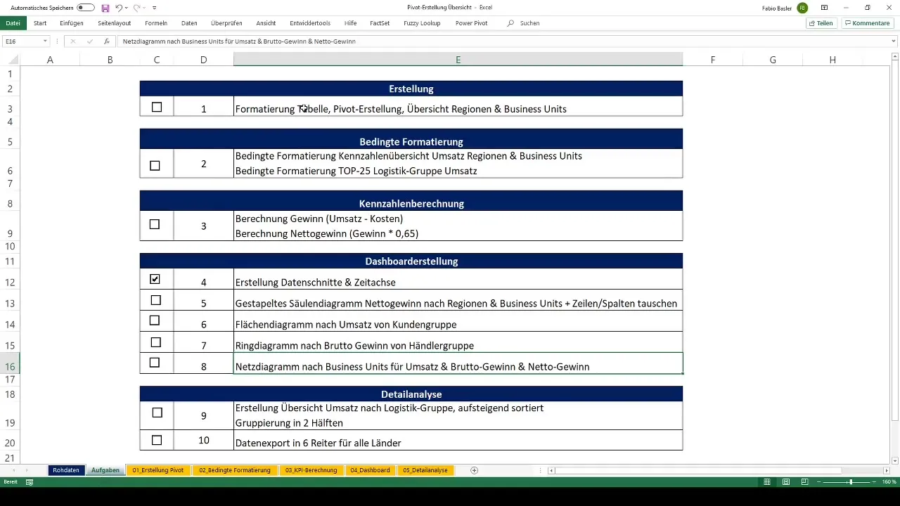
1. Prepare Raw Data

First, your task is to prepare your raw data and format it as a table. In the example, you can use the raw data you want to analyze in Excel. Make sure your data does not contain empty cells and that the headers are clearly visible. To format the data as a table, select the entire data range by pressing Ctrl + A. Then you can use the key combination Ctrl + T to create the table.

2. Create Pivot Table

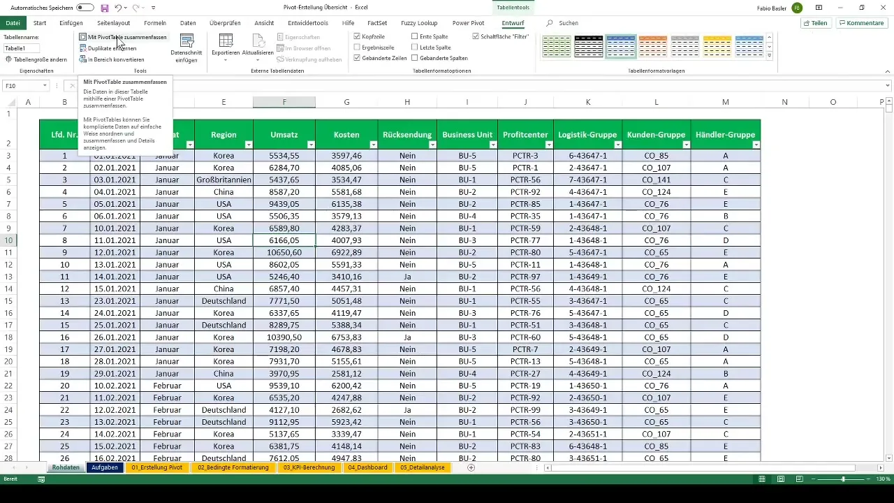
After formatting the raw data as a table, it's time to create the pivot table. Go to the Table Tools tab at the top in Excel. Here you will find the PivotTable option. Click on it and choose to create a new pivot table.

3. Confirm Input Form

In the input form for the pivot table, confirm everything with OK. This will start the initial pivot analysis. From now on, your pivot table will be referred to as PivotTable 1. You can customize the name as you wish.

4. Structure Data

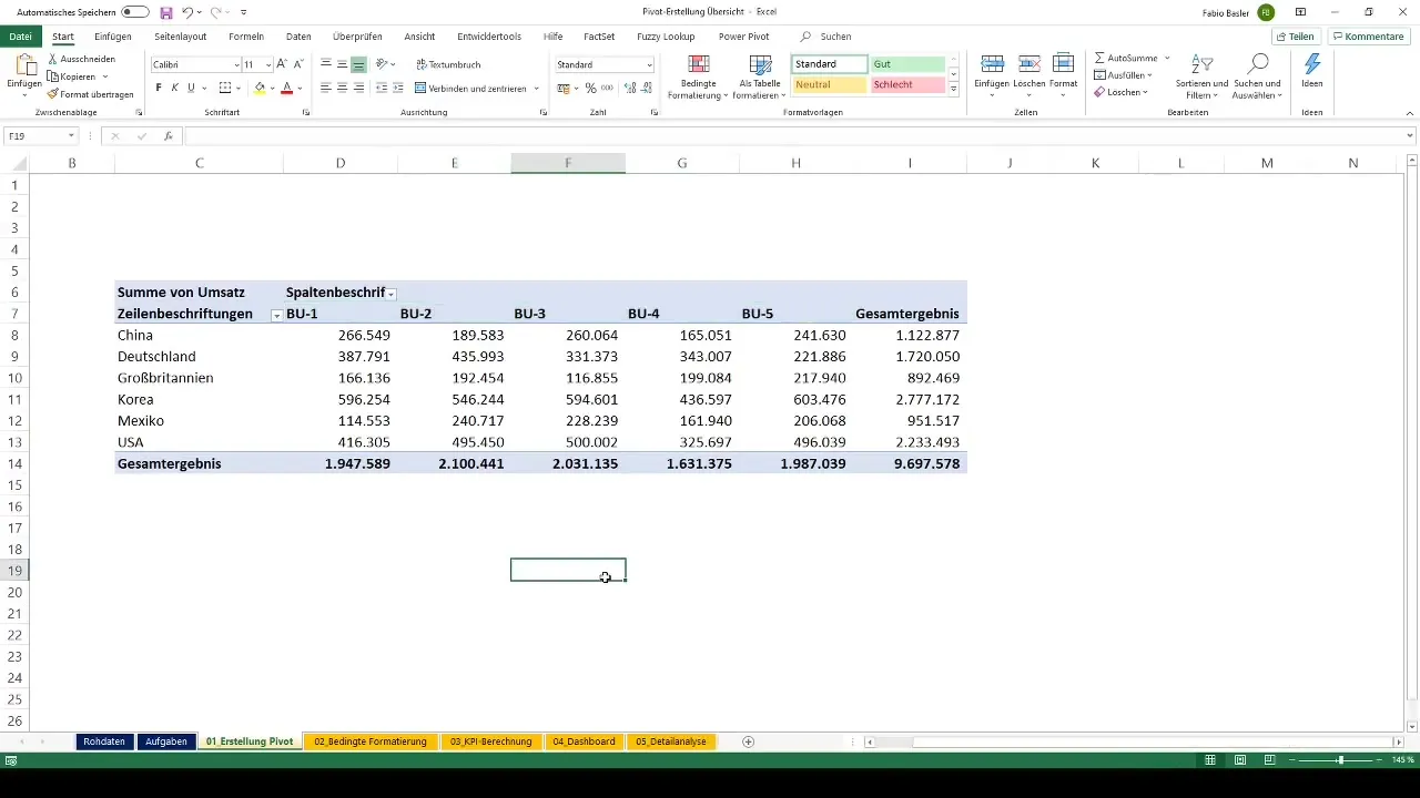
Now comes the next step: you want to break down the sales by regions and business units. Drag the Regions into the Rows area and the Business Units into the Columns area of the pivot table. Then drag the Sales into the Values area.

5. Adjust Automatic Formatting

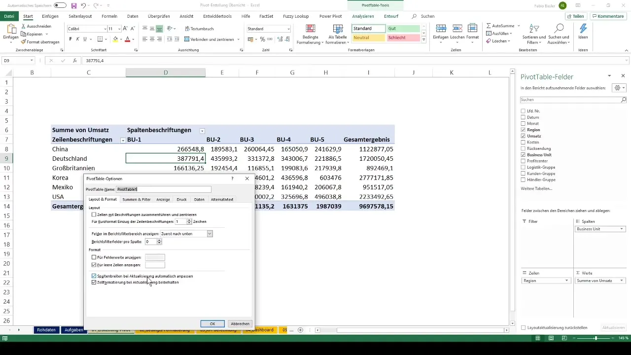
One small detail you may want to adjust is the automatic column formatting. You can do this by right-clicking on the pivot table and selecting PivotTable Options. Uncheck the option AutoFit Column Width on Update. This way, you can make the columns wider or narrower without Excel overwriting it with each update.

6. Format Numbers

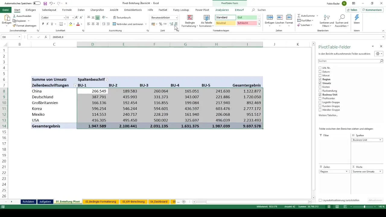
Now it's time to format the numbers in the pivot table to make them more readable. Add a thousand separator and remove the decimal places. This ensures that the numbers are easier to understand at a glance and present better.

7. Data Clarity

With these adjustments, you have already created a nice overview of sales by regions and business units. You can see the results for China, Germany, the United Kingdom, Korea, Mexico, and the USA, as well as for the individual Business Units (BU1 to BU5) at a glance.

Summary

In this guide, you have learned how to prepare raw data, create a pivot table, adjust the structure, and format the display accordingly. With these steps, you are able to create concise and clear analyses from your data.