Pivot tables in Excel: Data preparation and export

Welcome to this comprehensive guide where you will learn everything about data preparation, sorting, and exporting Pivot Tables in Excel. Pivot tables are a powerful tool for analyzing and visualizing data. This guide will take you through the final steps of a project where you have learned how to create and customize pivot tables to extract valuable information from raw data. By the end of this guide, you will be able to professionally process and present your data.

Main Insights

• You will learn how to prepare data in Excel.
• You will learn how to sort pivot tables according to specific criteria.
• The process of exporting data from pivot tables will be explained step by step.
• Groupings help with the clarity of the data.

Step-by-Step Guide

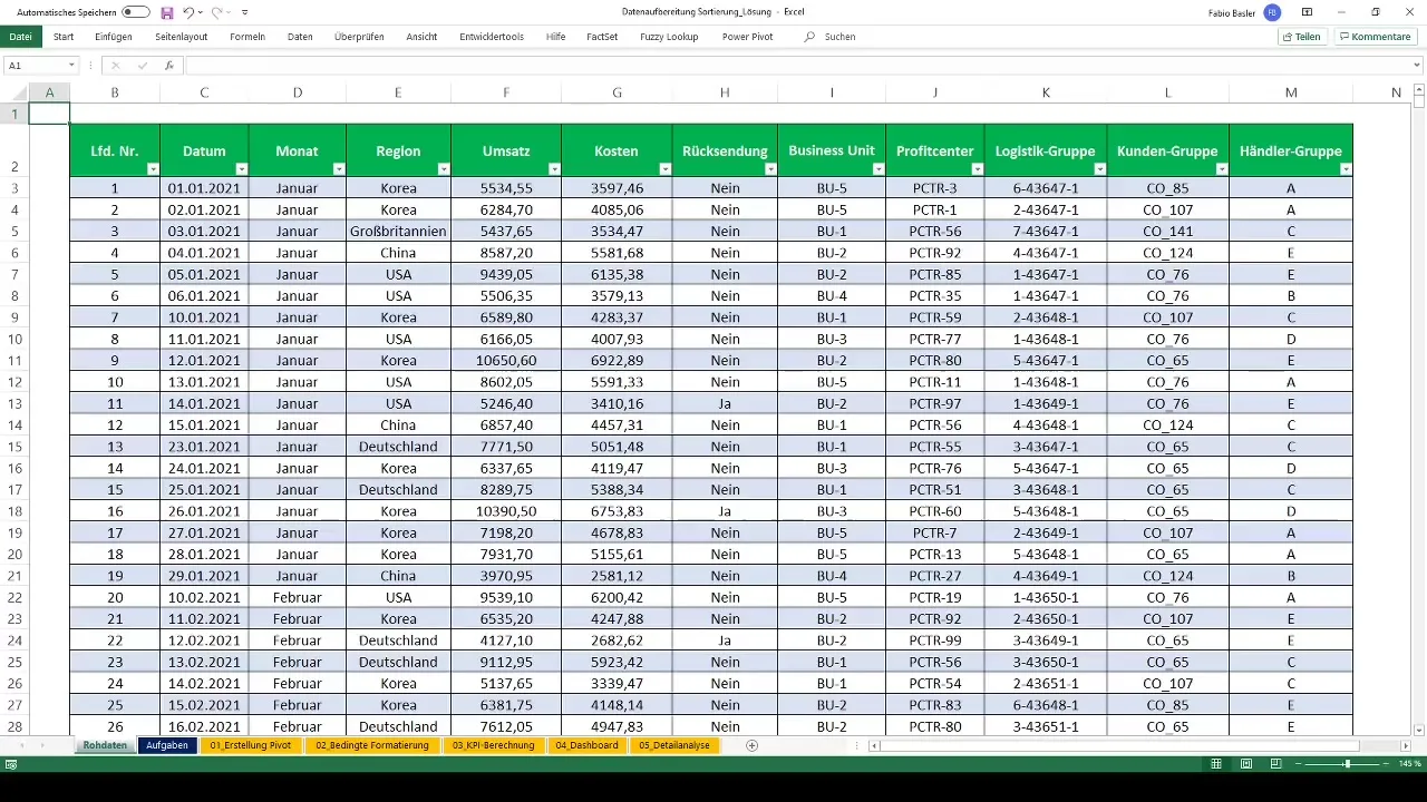
First, we need to insert the raw data into our Excel document. You can do this easily by going to the table where your data is stored. Then select the "Table Tools" function and choose "Pivot Table". This opens a new worksheet where you can create your pivot table.

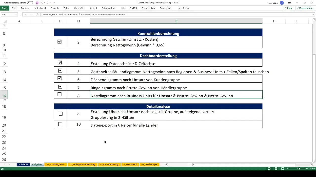
Next, you define the range where your pivot table should be placed. In our example, the numbers are positioned around row 5. To analyze the sales data efficiently, you drag the logistics groups into the row occupancy of the pivot table. It is important here that you format the values normally so that they are displayed as numbers with a thousand separator.

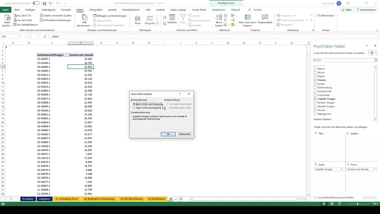
To make the pivot table neat and clear, you sort the expanded data. This can be done easily through the "Data" tab. There, you can then choose "Ascending Sort". This brings the lowest sales to the top of your analysis, helping you interpret the data more quickly.

Now, we want to group the data to analyze it even better. First, we check the number of values we have. In our example, we can do this by using the key combination Control + Shift + Arrow Up. This shows us that we have a total of 598 values. To group them evenly, we divide this number by 2, resulting in two groups of 299 values each.

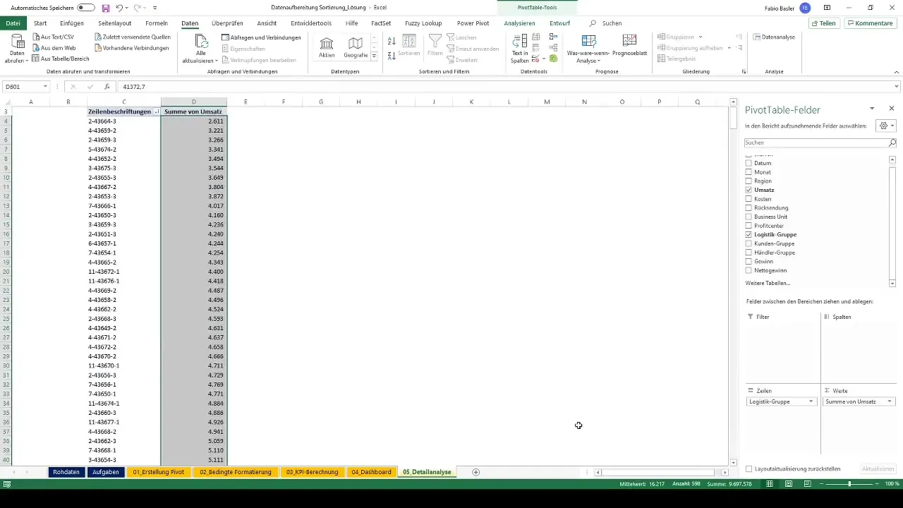
Highlight the first 299 values to create the first group. Then click on "Group Selection". This will organize the values into a clear structure. You can create the second group analogously by selecting the remaining values and also clicking on "Group Selection". Now you have two groups that significantly facilitate the analysis of the sales.

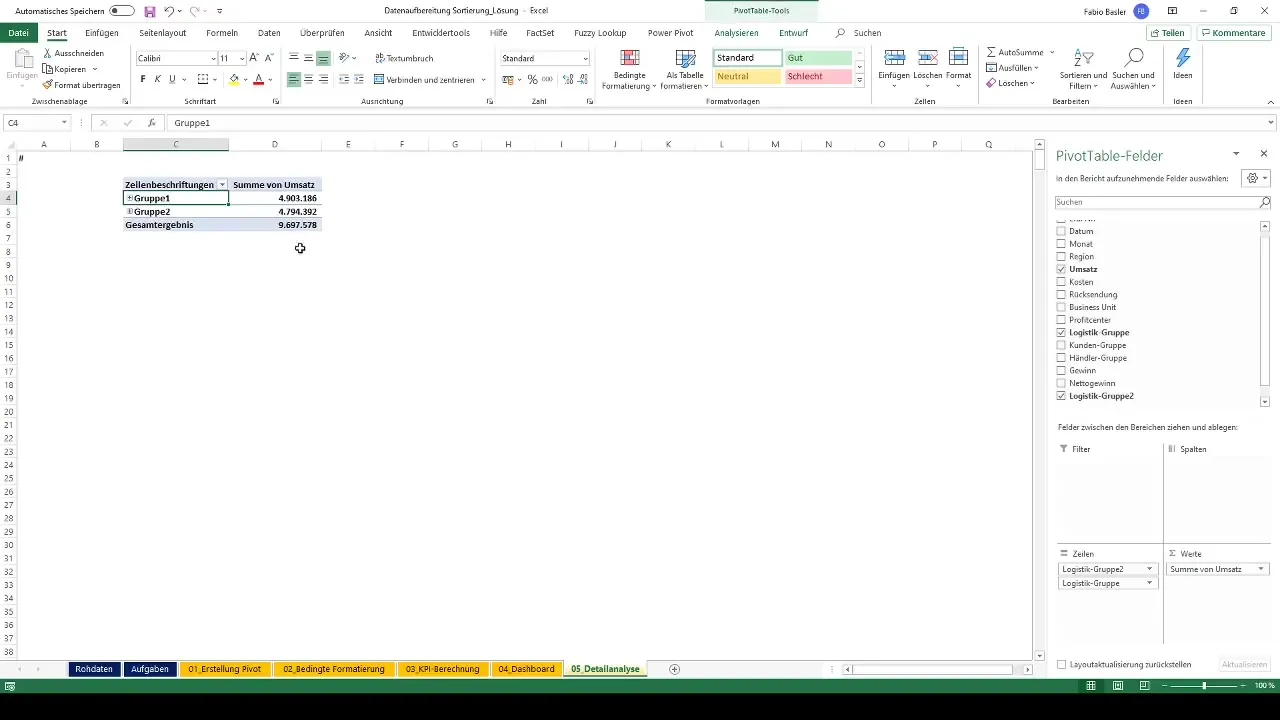
Next, we move on to the next task: data exporting. You want to export the results to different countries. This is also done through a new pivot table, which you create again with "Summarize PivotTable". Select the output area and drag the individual regions into the row view of the new pivot table. Now you can analyze the sales for each country.

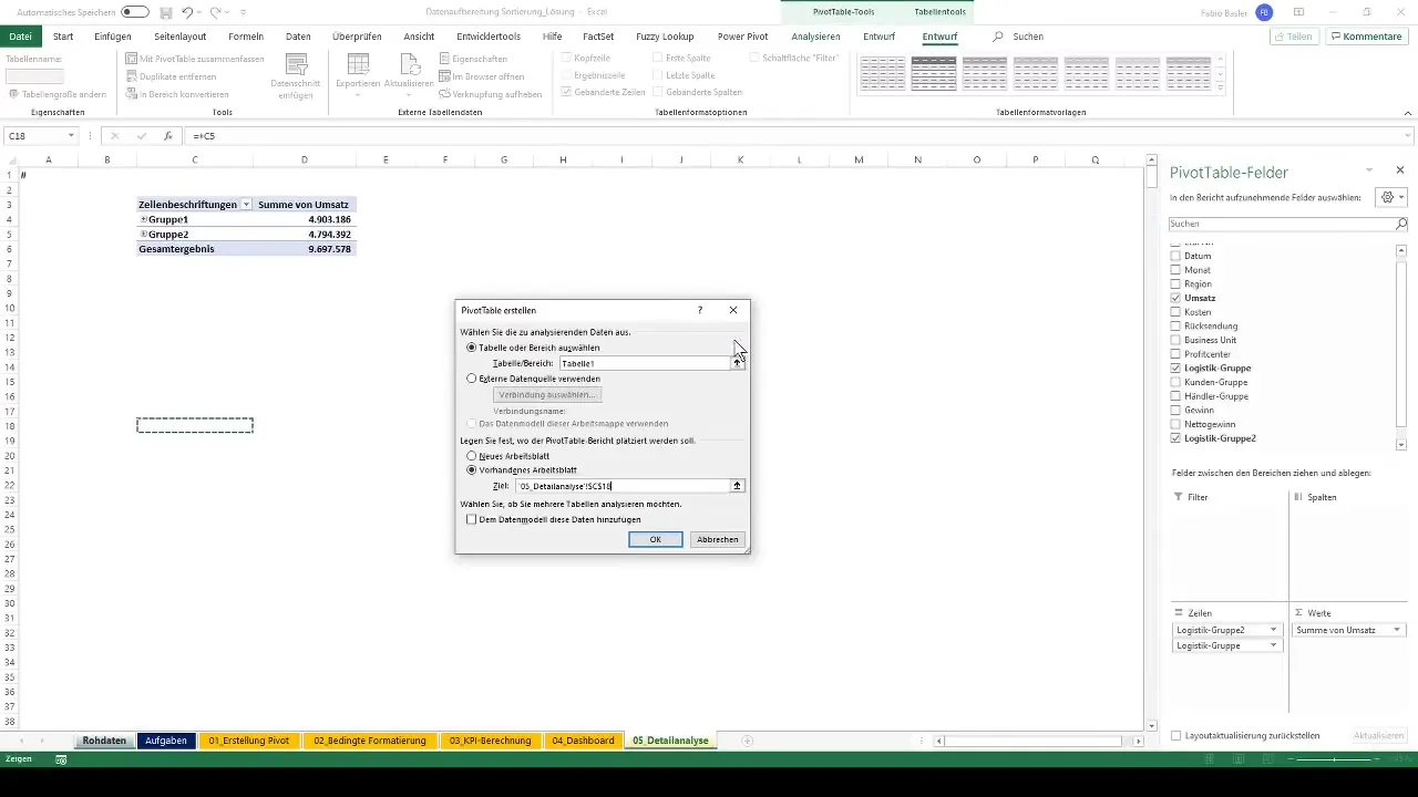
To create detailed reports for each country, simply double-click on the sales values in the pivot table. This will open a detailed view listing all relevant information, including sales, costs, and other dimensions. You can rename the individual reports to increase clarity.

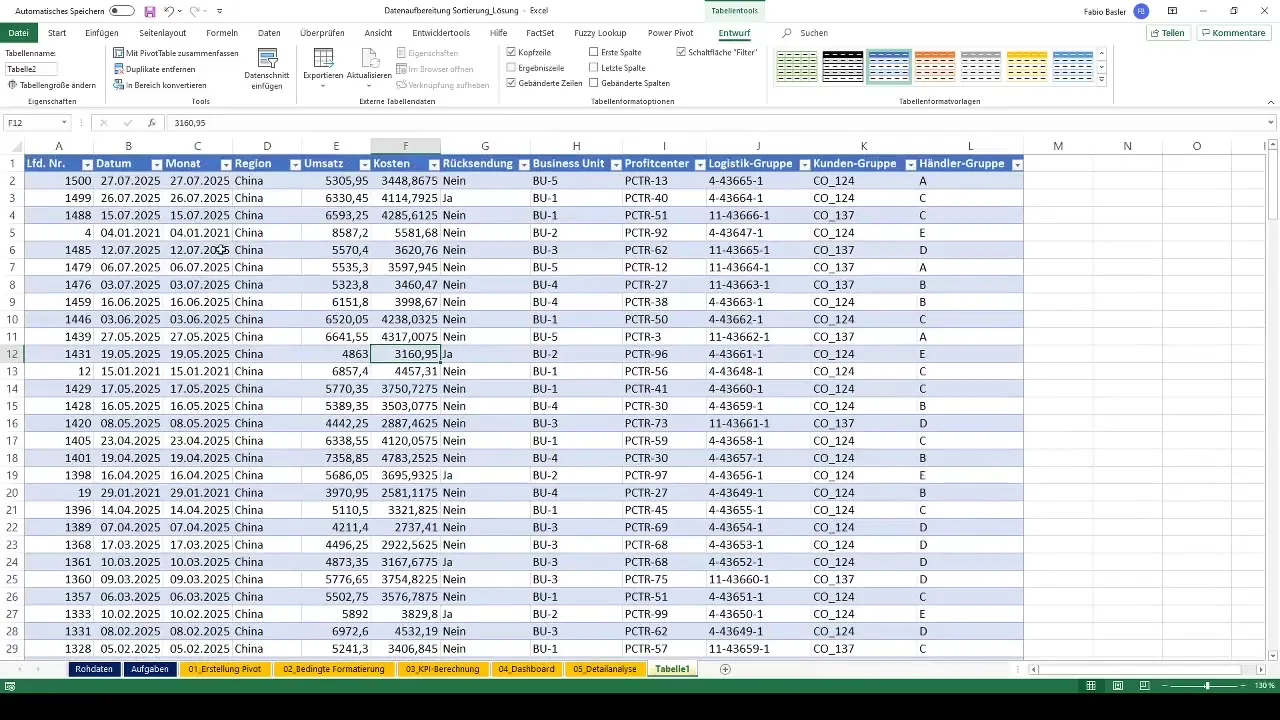
Repeat this process for the remaining countries and rename the respective reports. This method allows you to create customized information for various departments within your organization. Your colleagues can easily receive the report needed for their analyses.

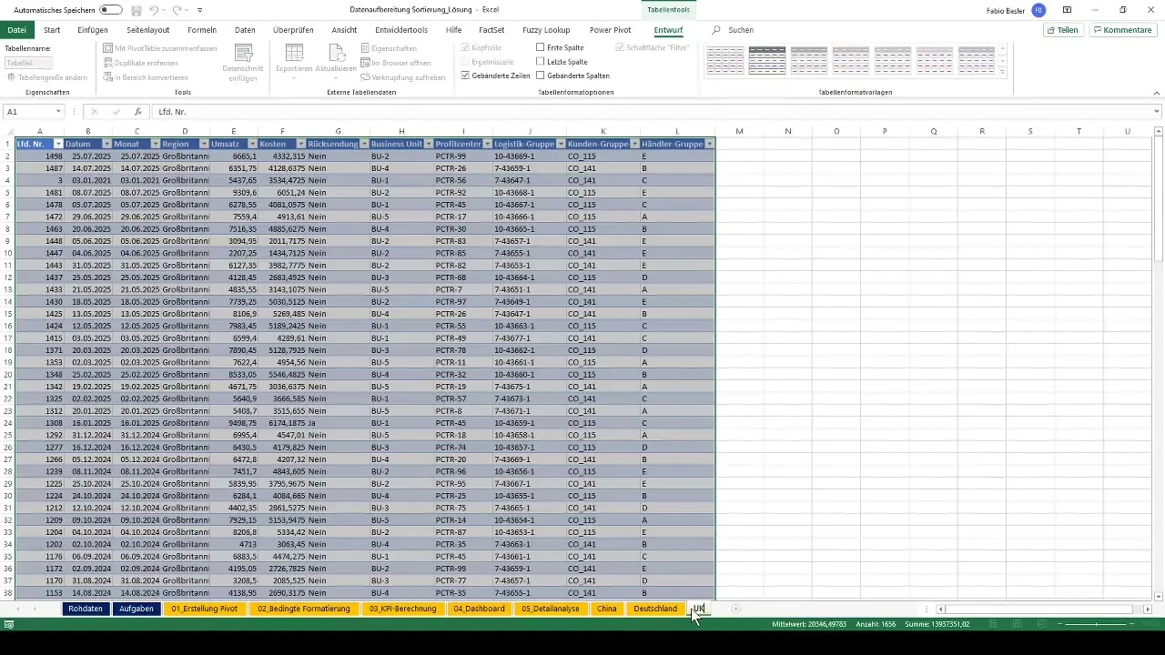
If you want to extract the desired data for a specific country, mark the relevant numbers and you can either export them to a new worksheet or a new Excel workbook. This way, you have the option to share this data with other departments.

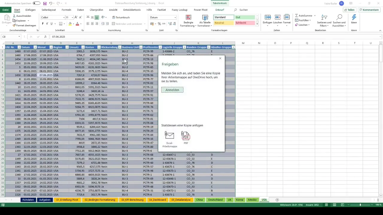
Finally, let's summarize the created reports. Utilize the option to summarize the data, which is by default formatted as a table, in a new pivot table. This way, you can quickly summarize all the necessary information about the individual countries.

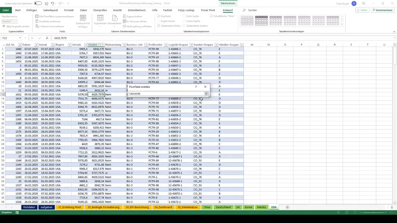
You have now successfully completed all the tasks. Go through the steps again to strengthen your knowledge and become an expert in pivot tables in Excel. It was a pleasure guiding you through this lesson, and I hope you were able to gain a lot from this tutorial.

Summary

In this tutorial, you have learned the method of data preparation, sorting, and exporting pivot tables in Excel. With these skills, you can efficiently analyze and present data.