Understanding conditional formatting in pivot tables

This guide focuses on conditional formatting in Pivot tables in Excel. Conditional formatting is a powerful feature for visually representing data and quickly identifying trends and outliers. In this tutorial, I will show you how to create two different conditional formats for your Pivot tables. We will organize the sales data by regions and business units, as well as by individual logistics groups, and highlight the key metrics accordingly.

Key Insights

• Conditional formatting allows for visual analysis of Pivot data.
• The green-yellow color scale for representing sales values.
• Applying conditional formatting to specific data points.

Step-by-Step Guide

Let's start with the first task, which involves creating a Pivot table that breaks down sales.

First, you need to have your data organized and ready in Excel. You can either create a new Pivot table or copy an existing one that already has the necessary metrics. Here, we will initially work with an existing Pivot table. Go to the "Conditional Formatting" folder and copy the existing Pivot table that shows the overview by regions and business units.

Now that we have the Pivot table ready, let's focus on conditional formatting. This perspective is important as we want to highlight values for business units and countries in color. We use the sales perspective, where higher sales are more positive for the company. This provides the opportunity to use a simple green-yellow color scale to visually capture the values.

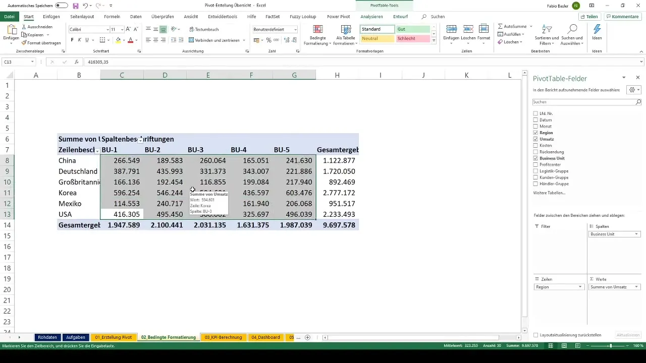
The idea is that the higher the sales value, the better it is. Therefore, we will represent higher sales in a greener shade, while lower sales will appear in yellow. This allows for a quick visual interpretation of the key values.

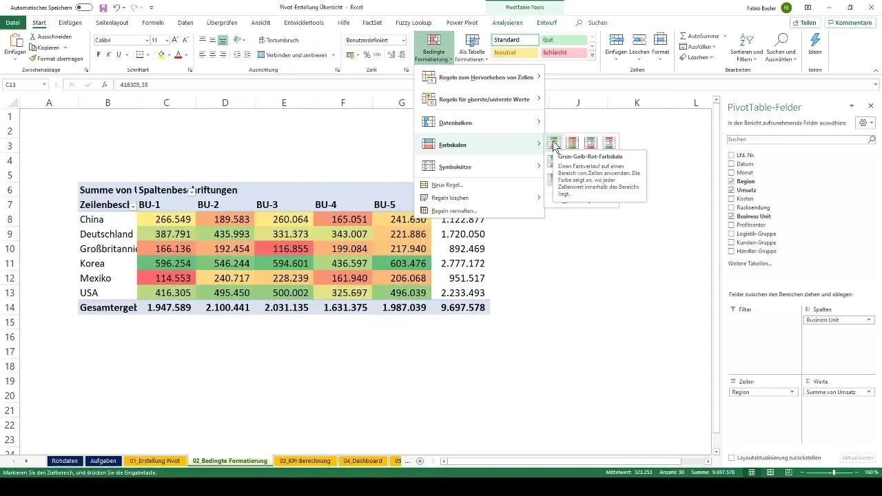
Let's now look at the result. An example is Korea in Business Unit 5 with sales of 603,000 euros, which is the highest value. In addition, there are sales from Mexico and the UK, which are relatively lower, allowing you to quickly recognize the performance of each region.

Now let's move on to the second overview, which breaks down sales by logistics groups. Here too, we will create a new Pivot table. Go to the Pivot Table Tools and select "Summarize Pivot Table." Export the Pivot table to your existing "02 conditional formatting" worksheet.

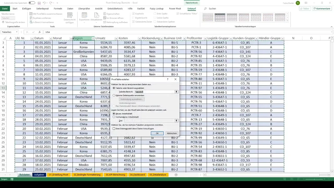
The goal is to present sales data structured by logistics groups. Once you have dragged the logistics groups into the rows, detailed overview should be available. This shows you all data clearly and understandably.

After creating the overview, it is important to format the data accordingly. Format the numbers to display the Euro symbol and use a thousand separator. But don't forget to remove the decimal places for clarity.

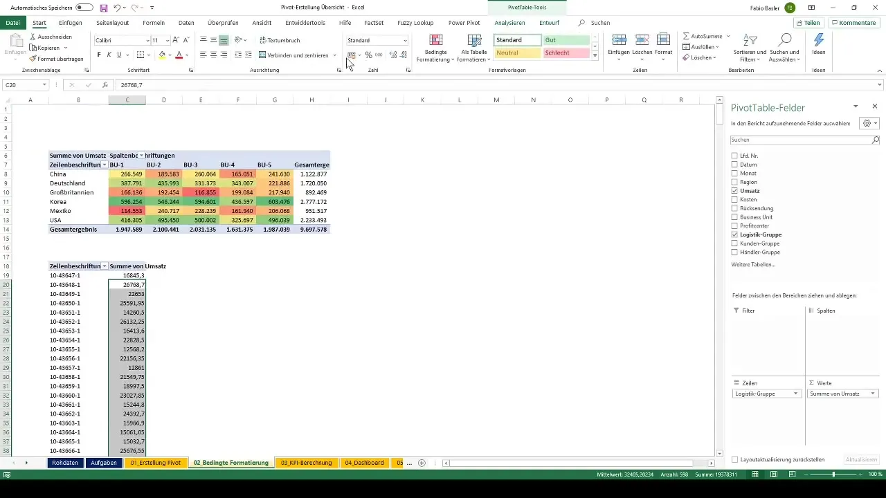
Once that is done, let's focus on the conditional formatting for the top 25 sales values. Go to conditional formatting and select the rule for the top 25 items.

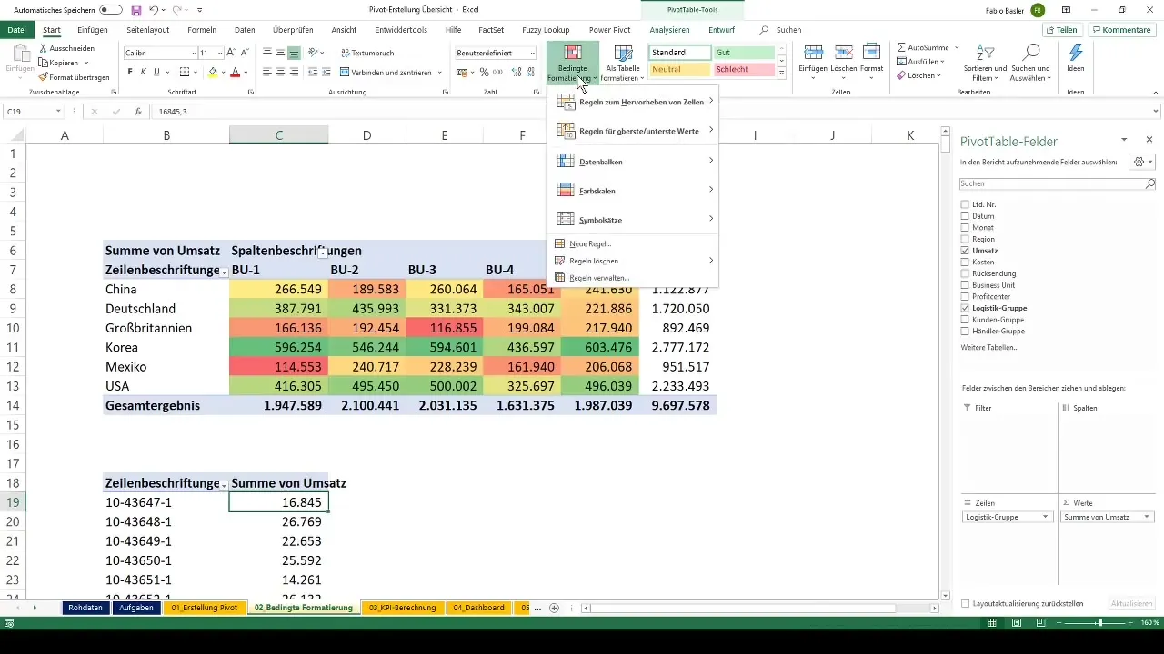
Mark these 25 values with a green fill. By clicking on the formatting options symbol, you can add the rule "All cells with sums of sales values for logistic group." This will filter out the logistic group based on the highest sales values and color it green accordingly.

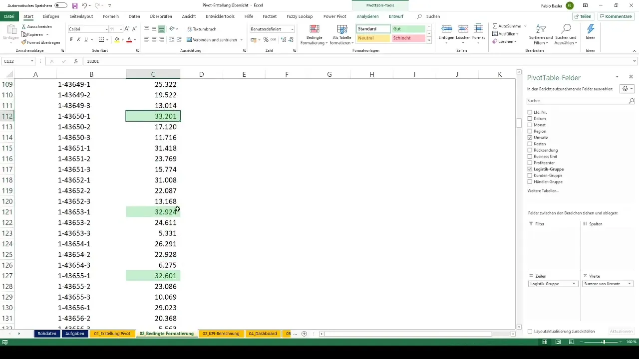
Once everything is set up and formatted correctly, you will be able to visually identify the top 25 sales values in your Pivot table, helping you quickly gain important insights into the sales performance of your logistics groups.

Summary

In this tutorial, you have gained a comprehensive overview of conditional formatting in pivot tables. You have learned how to visually enhance revenue data and how to apply a simple color scale to highlight key metrics. With the help of these techniques, you are now able to analyze your data more effectively and quickly identify trends in your pivot tables.