Pivot tables in Excel - effective data analysis

To take your analyses in Excel to a new level, pivot tables are essential. In this guide, you will learn how to conduct a comprehensive pivot analysis that provides valuable insights into your data. We will walk through the steps necessary to create and analyze various metrics from a given dataset.

Main Findings

• Using pivot tables allows for flexible data analysis.
• Calculations in pivot tables provide immediate results for revenue and profit.
• Detailed analysis allows for filtering and exporting specific datasets.
• Grouping data can help create a clearer overview.

Step-by-Step Guide

Step 1: Creating the Pivot Table

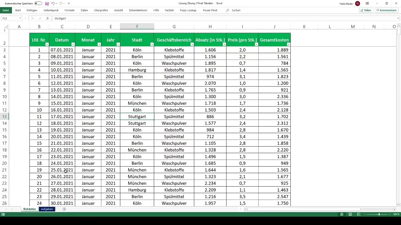
Begin by creating your pivot table. To do this, open Excel and select your data. You can quickly do this by pressing Ctrl + A and then Ctrl + T to select and format everything. Then, create the pivot table using the "Summarize with PivotTable" option, and position it in a new worksheet that you can name "Pivot Analysis."

Step 2: Overview of Sales by Cities and Business Areas

Once the pivot table is created, take the initial steps to create an overview of sales. Drag the "Sales" field to the values and the "Business Areas" and "Cities" fields to the rows and columns. You should now be able to see a clear overview. To make the overview more readable, it is advisable to assign the cities and business areas accordingly.

Step 3: Calculating Revenue

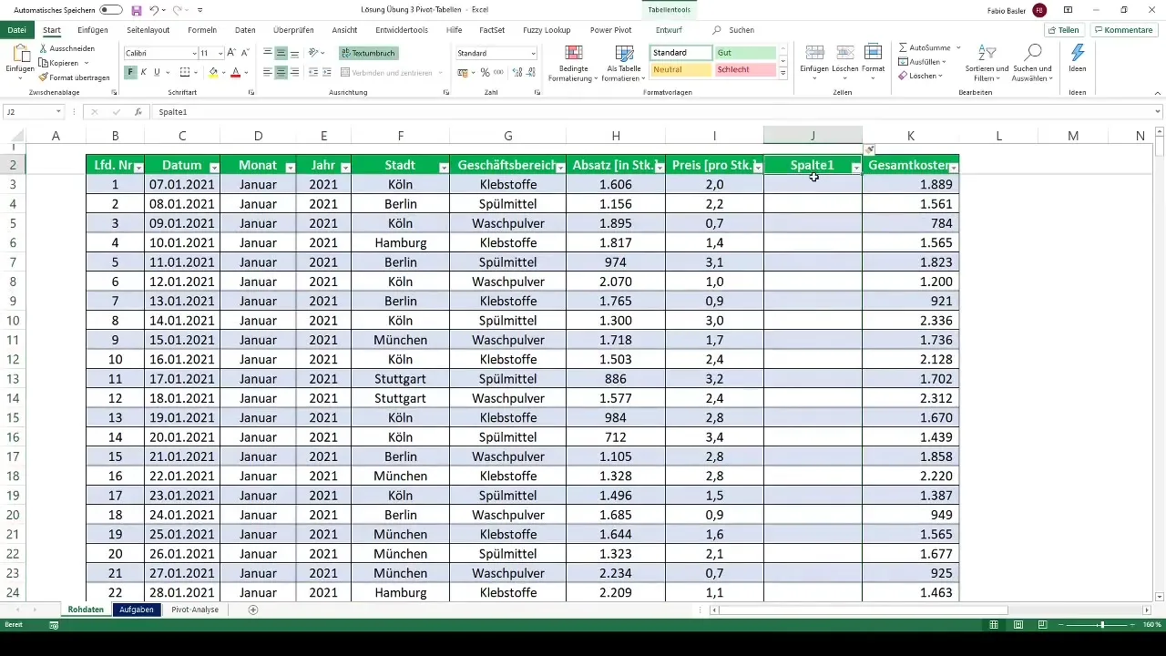
Now you can begin calculating revenue. This is done by multiplying the sales numbers by the unit prices. To do this, insert a new column by right-clicking and selecting "Insert Cells." Name the new column "Revenue" and calculate the revenue using the formula "Sales * Unit Price." Drag this formula down for all rows. This format ensures the table remains updatable.

Step 4: Determining Profit

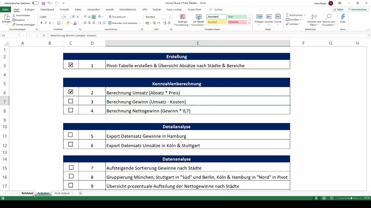
To calculate profit, you can create another column. Alternatively, you can also simply use the pivot options by creating a new pivot table and inserting the relevant fields for revenue and costs. Profit is calculated as "Revenue - Total Costs."

Step 5: Calculating Net Profit

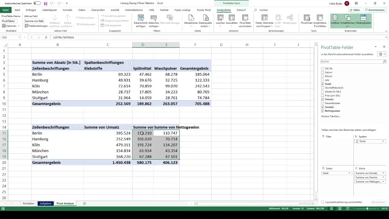
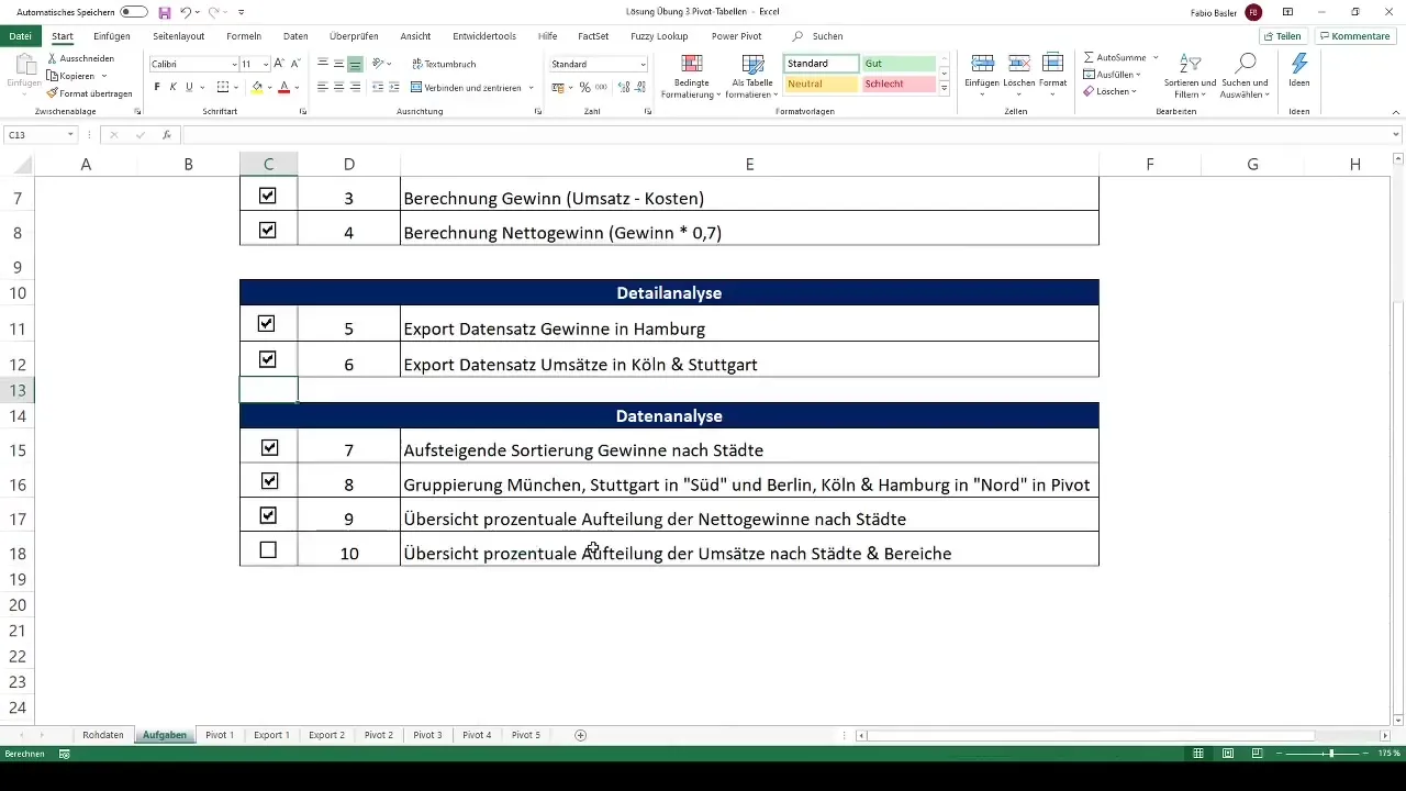
To calculate net profit, return to your pivot analysis. Click on "Analyze," then on "Field, Item & Set." Here, add net profit by taking the profit times 0.7, representing 70% of your total profit as net profit.

Step 6: Detailed Analysis through Export

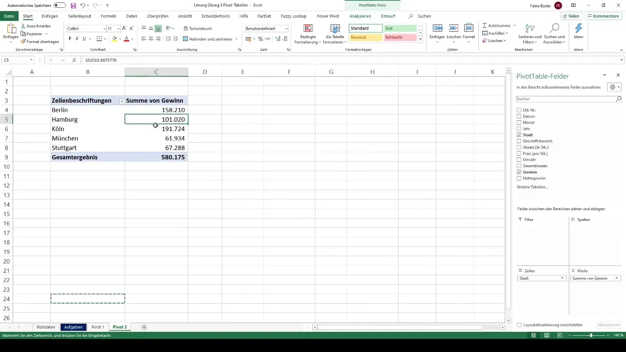
To create a detailed analysis, you can create a new pivot table and focus on gross profits per city. Remove the business areas from the pivot table and drag the "Profit" field into the values area. This way, you can get targeted information on sales regions, such as for Hamburg.

Step 7: Data Export for Revenues

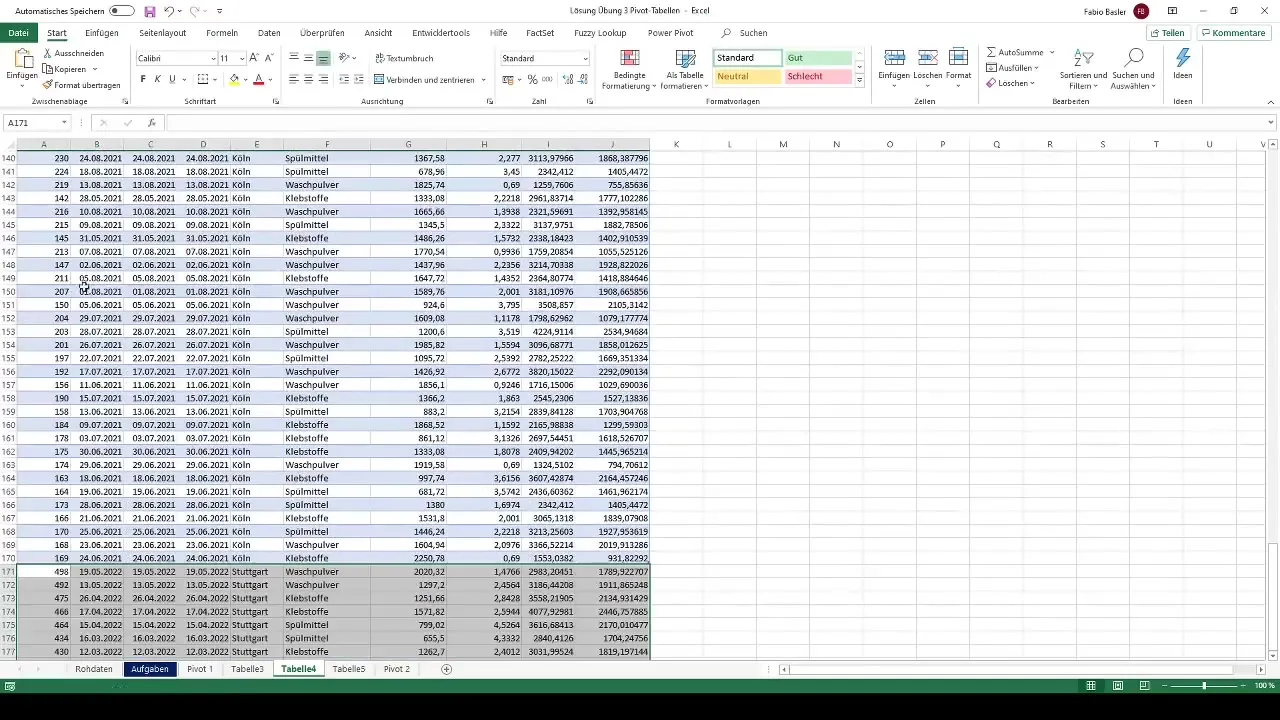
Now create another pivot table for data export. Copy the previous pivot table and focus on the revenues of the cities Cologne and Stuttgart. Double-click on the numbers of the cities to export the data. Make sure to organize and merge the data sheets accordingly.

Step 8: Sorting Profits

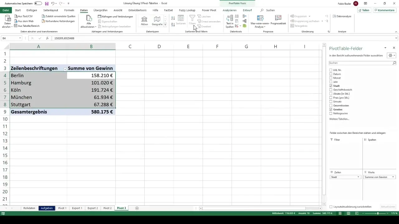
When analyzing profits, you may want to sort them in ascending order to better see how profits vary by cities. Create a new pivot table, drag profit into values and cities into rows. Then select the results, go to "Data," and sort as needed.

Step 9: Grouping the Cities

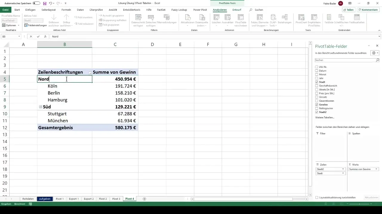
To create a better overview, you can group cities. For example, you can categorize Munich and Stuttgart into the "South" group, and Berlin, Cologne, and Hamburg into the "North" group. This is done by copying and adjusting the pivot table and using the grouping functions.

Step 10: Percentage Overview of Net Profits

To represent the net profits per city in percentage, create a new pivot table. Drag net profits and cities into the values and rows. Make sure to choose "% of grand total" in the value field settings to show the percentage shares.

Step 11: Percentage Representation of Revenues

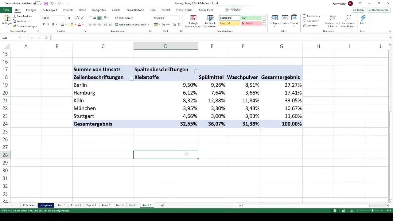
For the final task, copy the last pivot table and replace the net profits with revenues. Add the business areas and revisit the value field settings to represent the values as "% of grand total." You have now gathered all the essential information.

Summary

This step-by-step guide has shown you how to analyze and prepare complex data using pivot tables. From revenue to profit calculations, you have learned how to structure your data and gain deeper insights. Mastering these techniques can significantly enhance your Excel skills.