Working with pivot tables in Excel is an essential tool for anyone who regularly deals with data. In this guide, we show you how to calculate key figures to gain valuable insights into your data. In particular, we will focus on calculating profit and net profit. You don't need extensive expertise to understand and apply these steps. Let's dive right in!
Key Takeaways
- You will learn how to calculate key figures such as profit and net profit with pivot tables.
- The steps involve creating a new pivot table and using filtering and calculation functions in Excel.
- With the right formulas in Excel, you can easily analyze and interpret your data.
Step-by-Step Guide
To calculate your key figures using a pivot table in Excel, follow these simple steps:
Create a Pivot Table
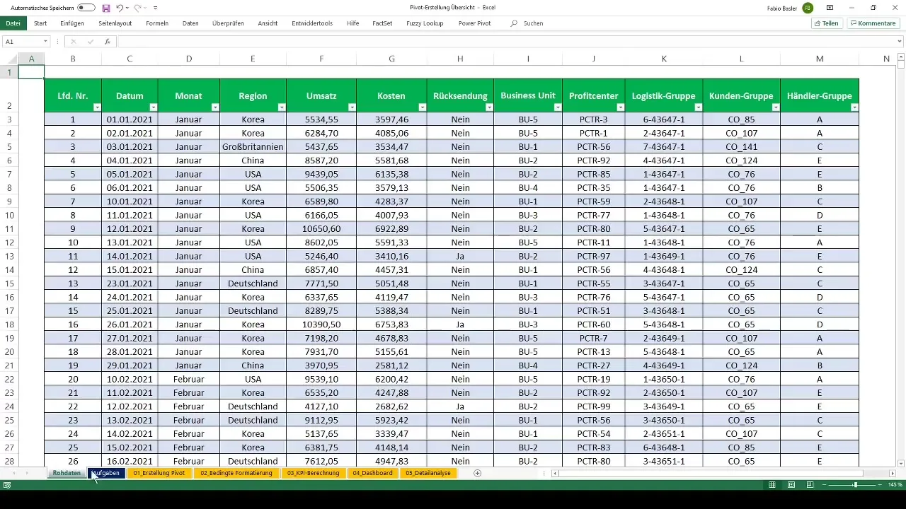
First, you need to create a pivot table to work with your data. Go to your existing worksheet where the revenue and cost data is stored. To create the pivot table, navigate to "Insert" and select "PivotTable." Then choose the data range you want to analyze.

Break Down Revenue by Business Units
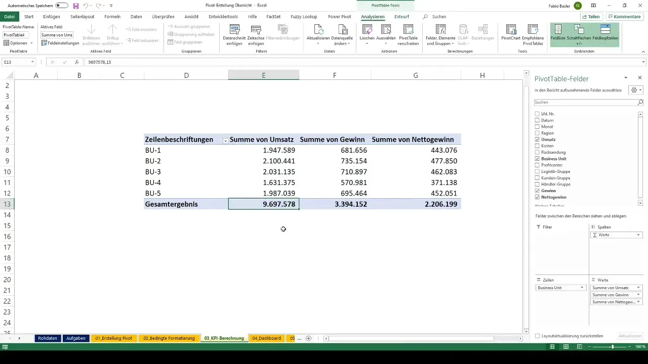
Now that your pivot table is created, you can analyze your revenue data. Drag the revenue metric into the value area of the pivot table. To sort the revenue data by individual business units, drag the corresponding column into the rows area. This will give you a clear overview of revenues by business unit.

Calculate Profit
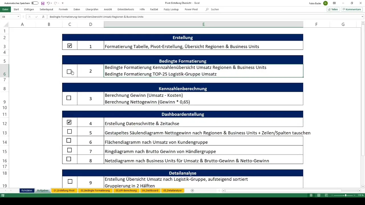
The next important metric you want to calculate is profit. Profit is calculated as follows: Revenue minus costs. To do this in the pivot table, go to "Analyze" and then "Fields, Items & Sets." Select "Calculated Field" to create a new field. Name it "Profit" and use the formula "Revenue - Costs."
Calculate Net Profit
To calculate net profit, we need to weight the profit. For this, we will assume a fictional tax rate of 35%. With this information, we can weight as follows: Net Profit = Profit (1 - Tax Rate). Go to "Analyze" again and choose "Fields, Items & Sets." Create another calculated field named "Net Profit." Set the formula accordingly to "Profit * 0.65."
Verify Results
Now you can verify your results. After creating both calculated fields, you will now see the revenue, profit, and net profit in your pivot table. It's important to keep the rounded values in mind; in this case, revenue is 9.7 million, profit is 3.4 million, and net profit after taxes is 2.2 million.

Summary
Using pivot tables in Excel to calculate key figures is an effective way to gain deeper insights into your data. You have now learned how to efficiently calculate profits and net profits and how important it is to use the right formulas to obtain realistic and useful results.
Frequently Asked Questions
How do I create a pivot table in Excel?To create a pivot table in Excel, go to "Insert" and select "PivotTable." Choose the data range and click "OK".
How do I calculate profit in a pivot table?Profit is calculated in a pivot table by creating a calculated field using the formula "Revenue - Costs."
How can I calculate net profit?Net profit is calculated by multiplying the profit by the factor (1 - Tax Rate). In this case, the tax rate is 35%.
How can I break down my pivot table by business units?Drag the Business Units column into the rows area of the pivot table to break down revenues by these units.
What are calculated fields in pivot tables?Calculated fields allow you to create new data fields based on formulas that you can apply to other fields in the pivot table.


