Data Analysis for Excel: Power Pivot Basics

Power Pivot gives you the ability to perform comprehensive analyses and create multidimensional data models from various data sources. In this text guide, you will learn the fundamental steps to use Power Pivot in Excel for your data analysis. You will see how to import data from different sources, integrate them into a data model, and then analyze them effectively. Get ready to take your Excel skills to the next level!

Key Insights

• Power Pivot allows importing and linking data from various sources.
• You can efficiently integrate data into a data model and perform multidimensional analyses.
• Modeling and establishing relationships between data sources are essential.
• Visualizations help understand and present analysis results better.

Step-by-Step Guide

Step 1: Activate Power Pivot

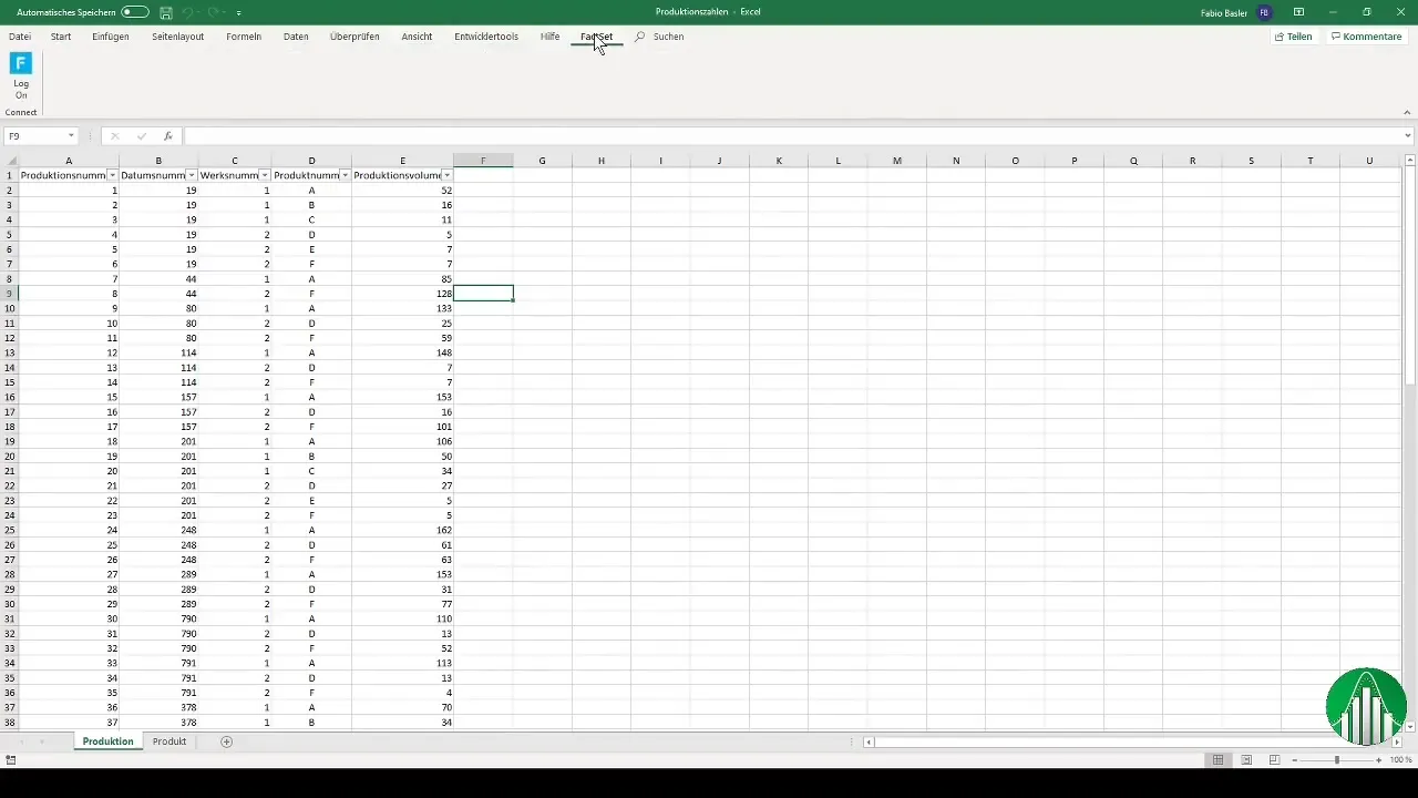
Before you can work with Power Pivot, you must ensure it is activated in your Excel. Go to the ribbon menu and click on "File". Then select "Options" and go to "Add-Ins". Here you will see a list of available add-ins. Look for "Power Pivot" and activate it.

Step 2: Prepare Data

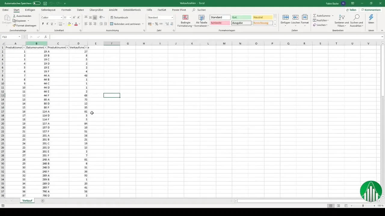
Open your Excel files containing the data for analysis. You should have at least two tables with production and sales figures. Additionally, you can use a CSV file and an Access database. This way, you have prepared different data sources.

Step 3: Format Data as Tables

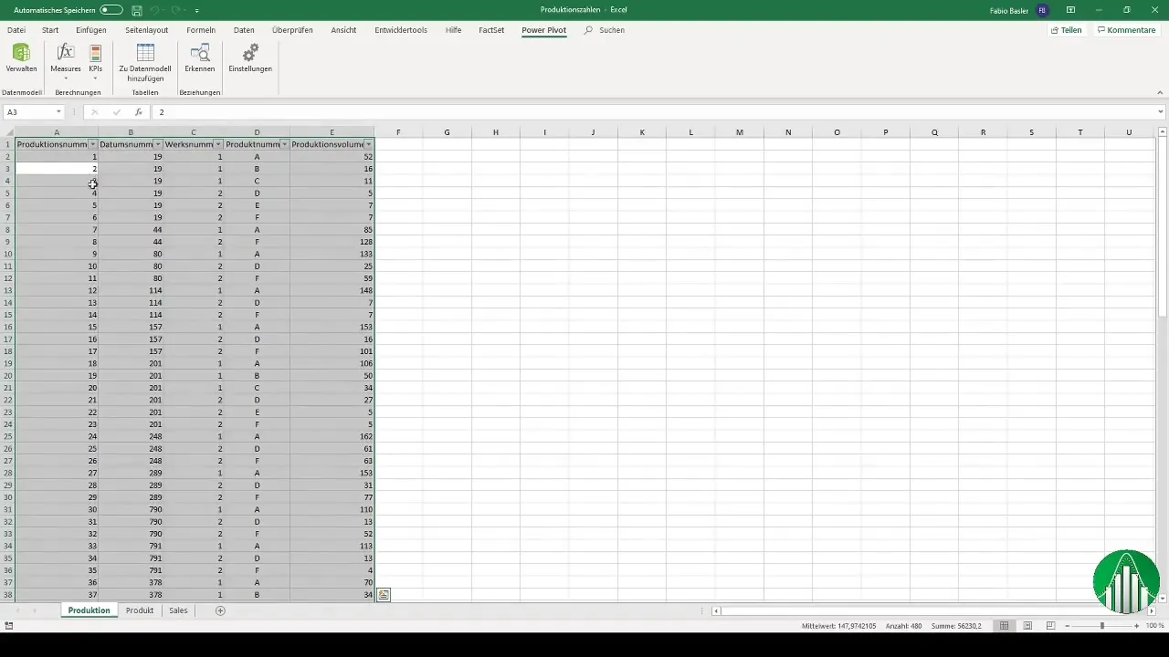
To ensure Excel recognizes the data correctly, you need to format each data row as a table. Select the relevant data and press "Ctrl + A" to select all cells. Then press "Ctrl + T" to format the selection as a table.

Step 4: Import Data into Power Pivot Model

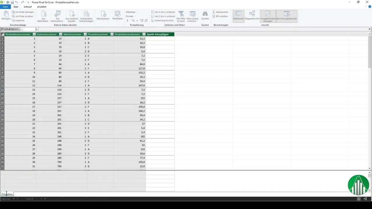
After formatting your data, you can import it into Power Pivot. Open the Power Pivot window and click on "Data Model". There, select the table you want to import and name it accordingly, for example, "Production", "Product", or "Sales" for sales figures.

Step 5: Import Additional Data Sources

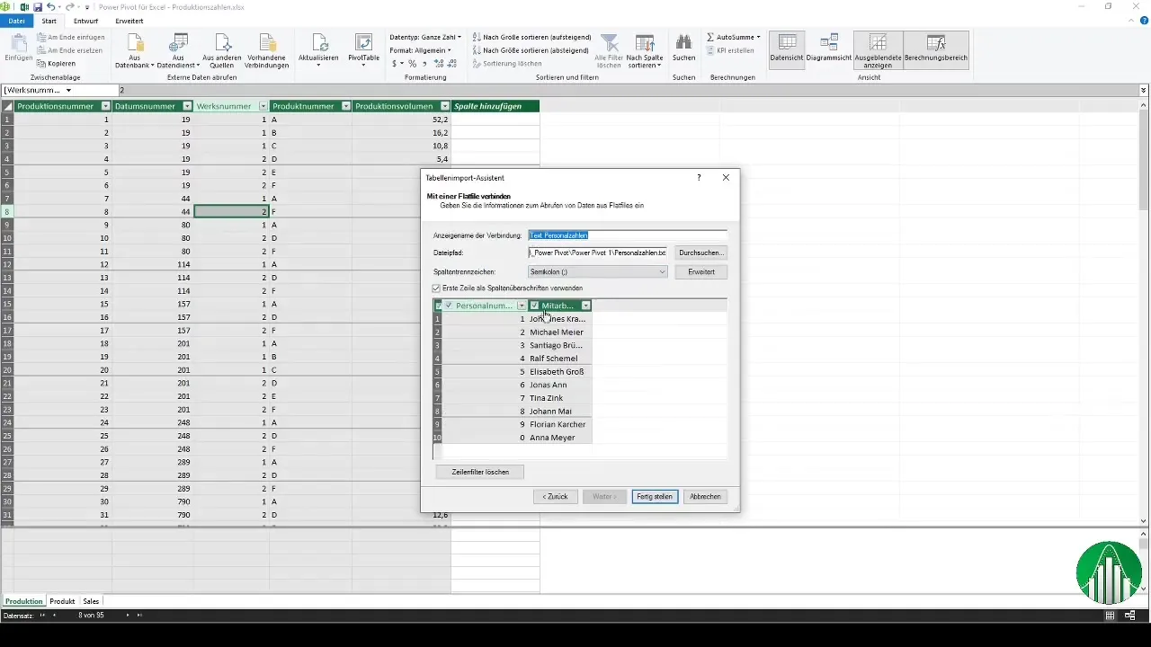
You can import more data from CSV files or databases. Click on "Import Data" and select the option that fits your data source. For instance, choose a text file, specify the delimiter (e.g., semicolon), and successfully import the data.

Step 6: Define Relationships Between Data

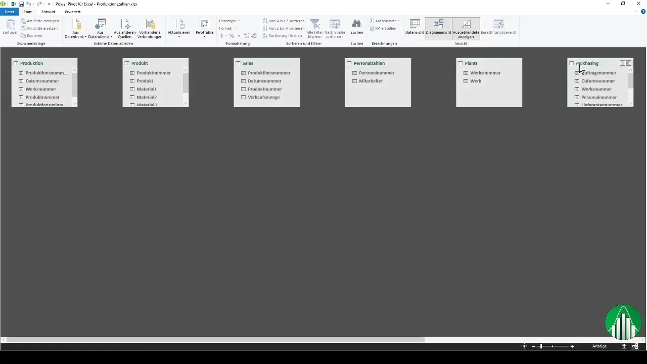
After importing your data, you need to establish relationships between different dimensions. Switch to the diagram view in Power Pivot and draw lines between the different fields to show how they are interconnected, such as between date numbers or product numbers.

Step 7: Perform Multidimensional Analysis

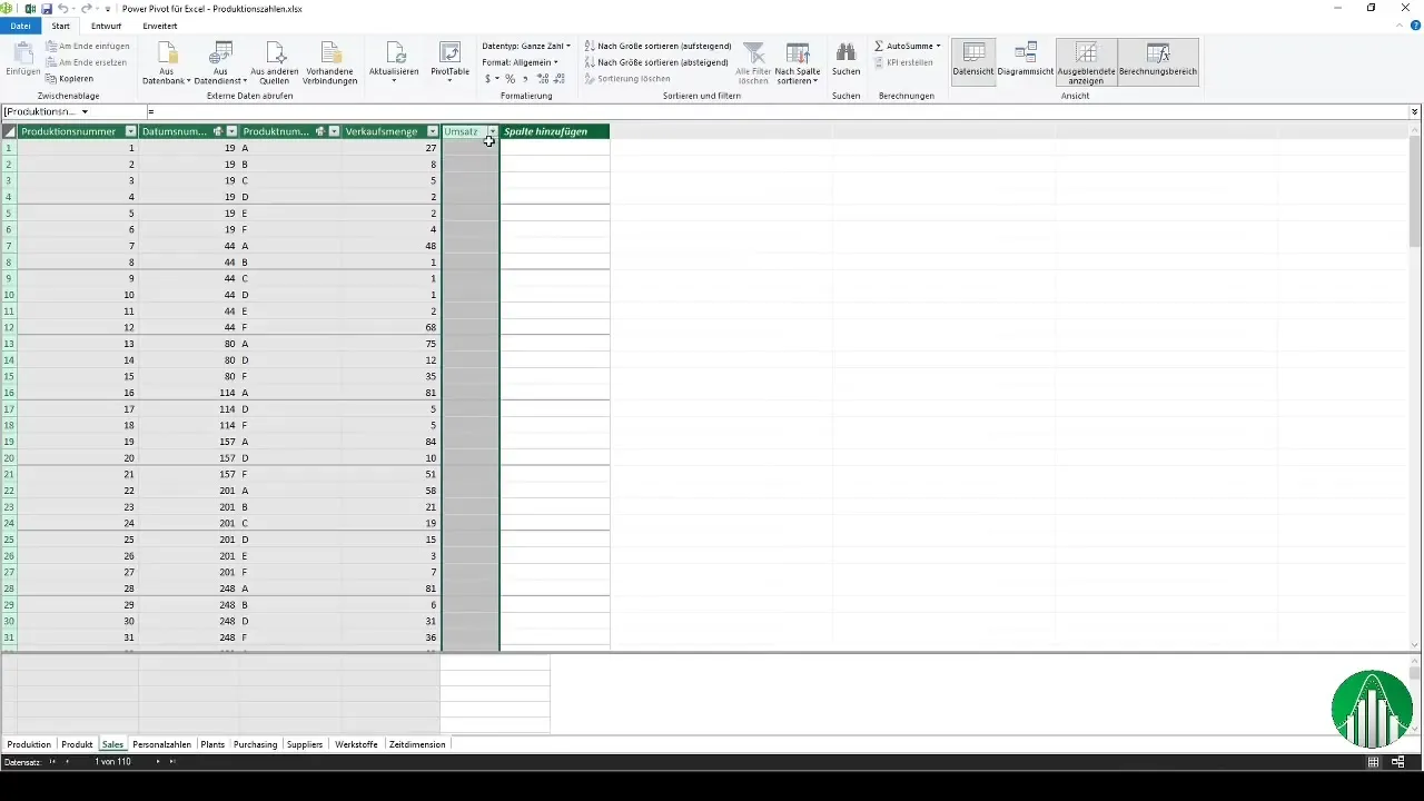
To analyze the data, return to the data view. Here, you can create your own metrics. For example, you can calculate revenue by multiplying sales quantity by price. This can be done across dimensions, allowing for a deeper analysis.

Step 8: Create PivotTable

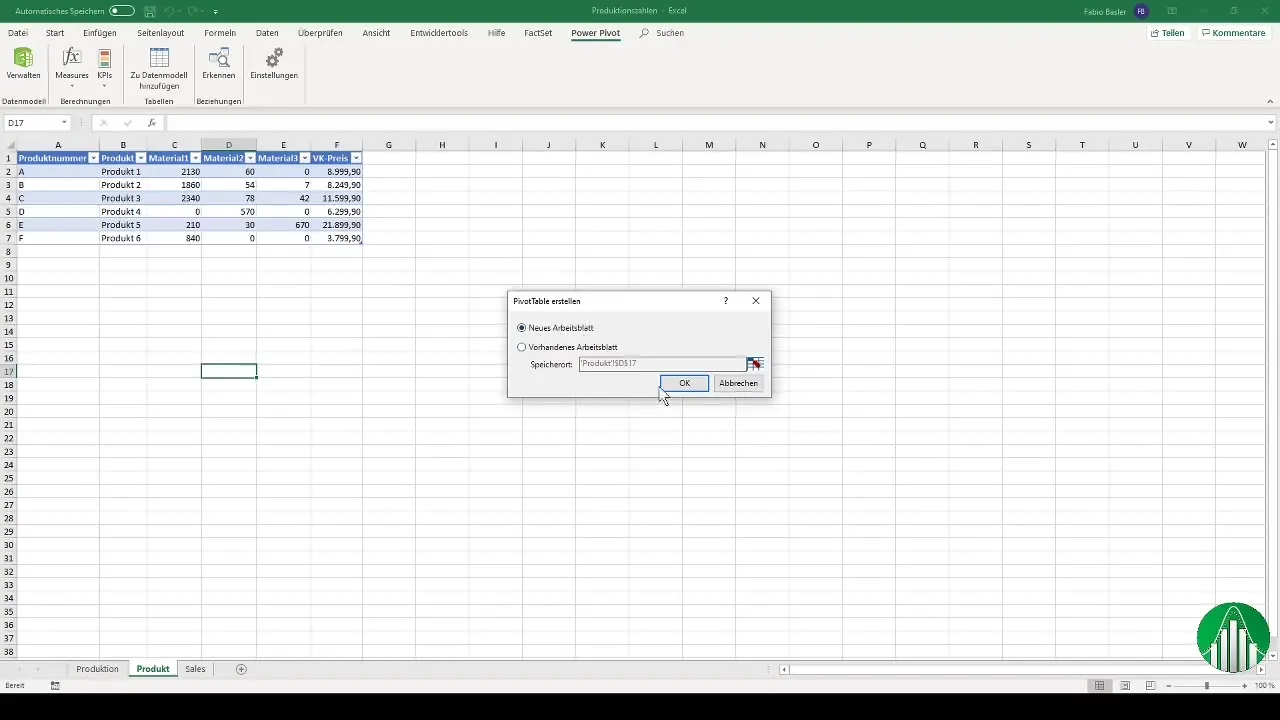
Create a PivotTable to visualize your data. Click on "Insert" and select the PivotTable option. Here, you can drag and drop fields to shape the analysis. What's special about Power Pivot is that you can create multidimensional reports from different dimensions.

Step 9: Creating charts for data visualization

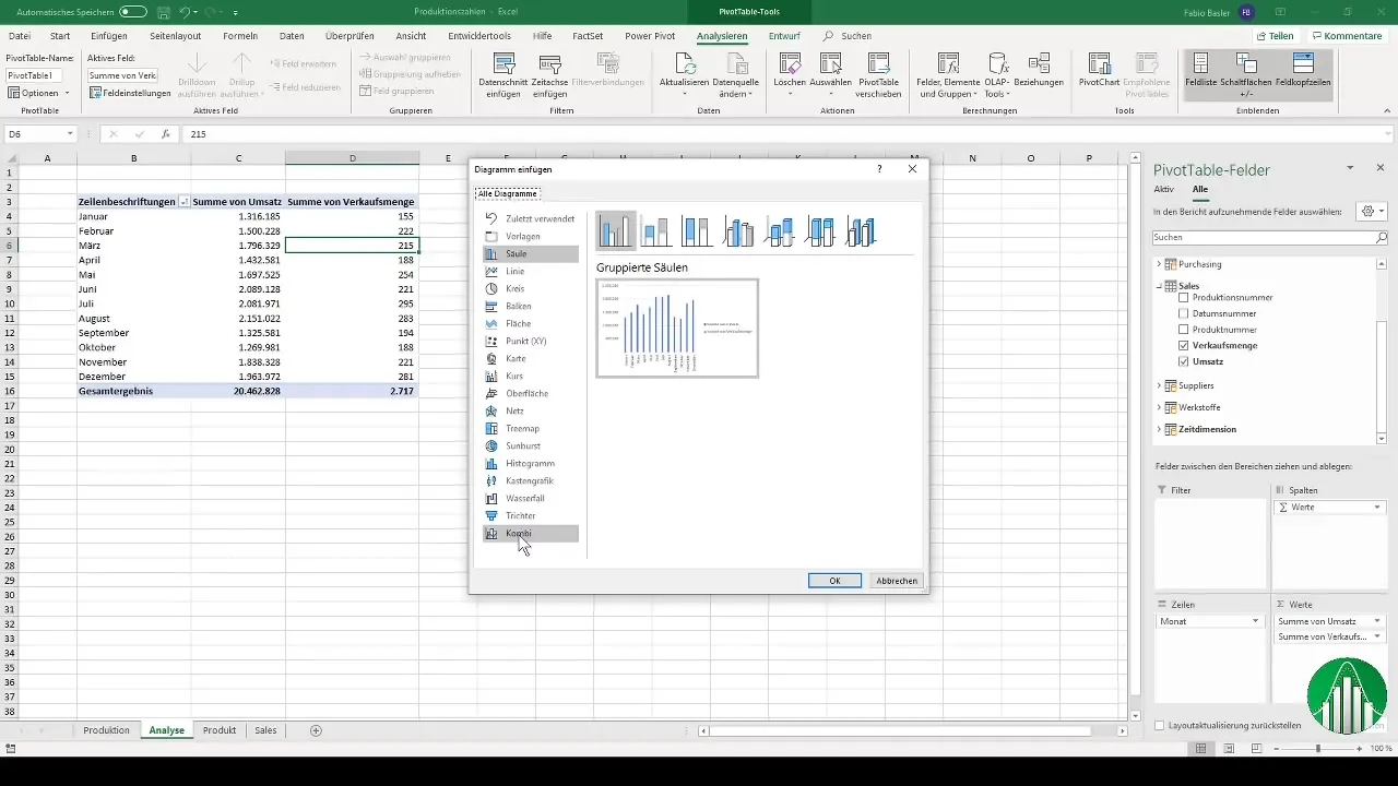
To make your analysis results more visual, you can add charts. To do this, select the chart options in the PivotTable Tools. This way, you can create grouped columns or combination charts, and present your data visually appealingly.

Step 10: Adding slicers

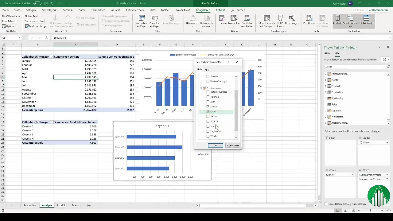
For better data analysis and navigation, you can add slicers. This way, you can filter the data by clicking and perform targeted analyses. For example, add slicers for months, quarters, or product numbers.

Step 11: Creating dynamic dashboards

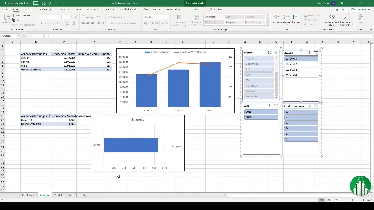
Use the capabilities of Power Pivot to create dynamic dashboards. This way, you can structure your data as in a reporting tool and adjust it accordingly.

Step 12: Presentation of results

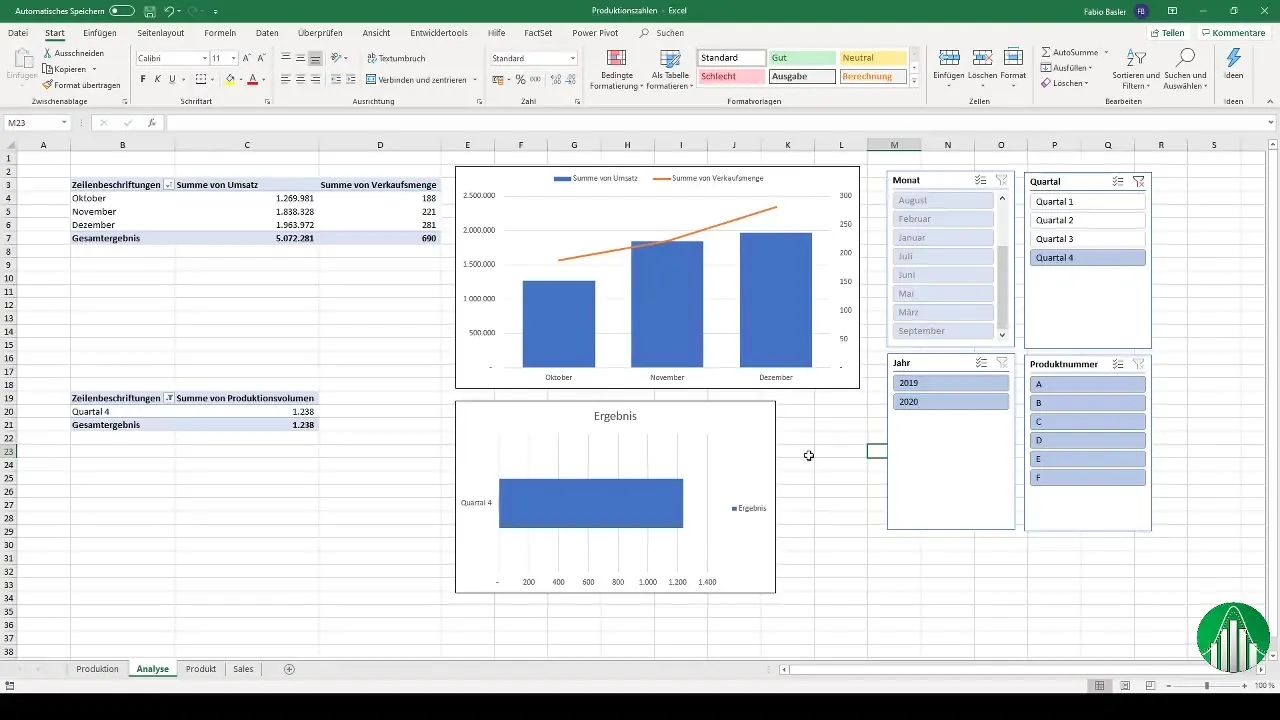
Finally, you can customize your dashboard to ensure that it not only informative but also visually appealing. Optimize the layout and present your results accordingly.

Summary

In this tutorial, you have learned how to activate Power Pivot in Excel, import data, and model effectively. You now also know the steps to perform multidimensional analyses and visualize them. With these skills, you are well equipped to take your data analysis to the next level.