Create and analyze pivot tables in Excel

You are facing the challenge of efficiently analyzing and presenting complex data in Excel? Pivot tables are one of the most powerful tools to achieve this. In this guide, you will learn how to create a pivot table using a practical example, calculate key figures, and perform basic data analyzes. You will gain a better understanding of the structure and functionality of pivot tables and be able to apply them to your own projects.

Key Insights

• You will learn how to create a pivot table in Excel.
• You will calculate key figures such as revenue and net profit.
• You will gain knowledge about detailed analysis and basic data analysis options.

Step-by-Step Guide

Step 1: Prepare Dataset and Create Pivot Table

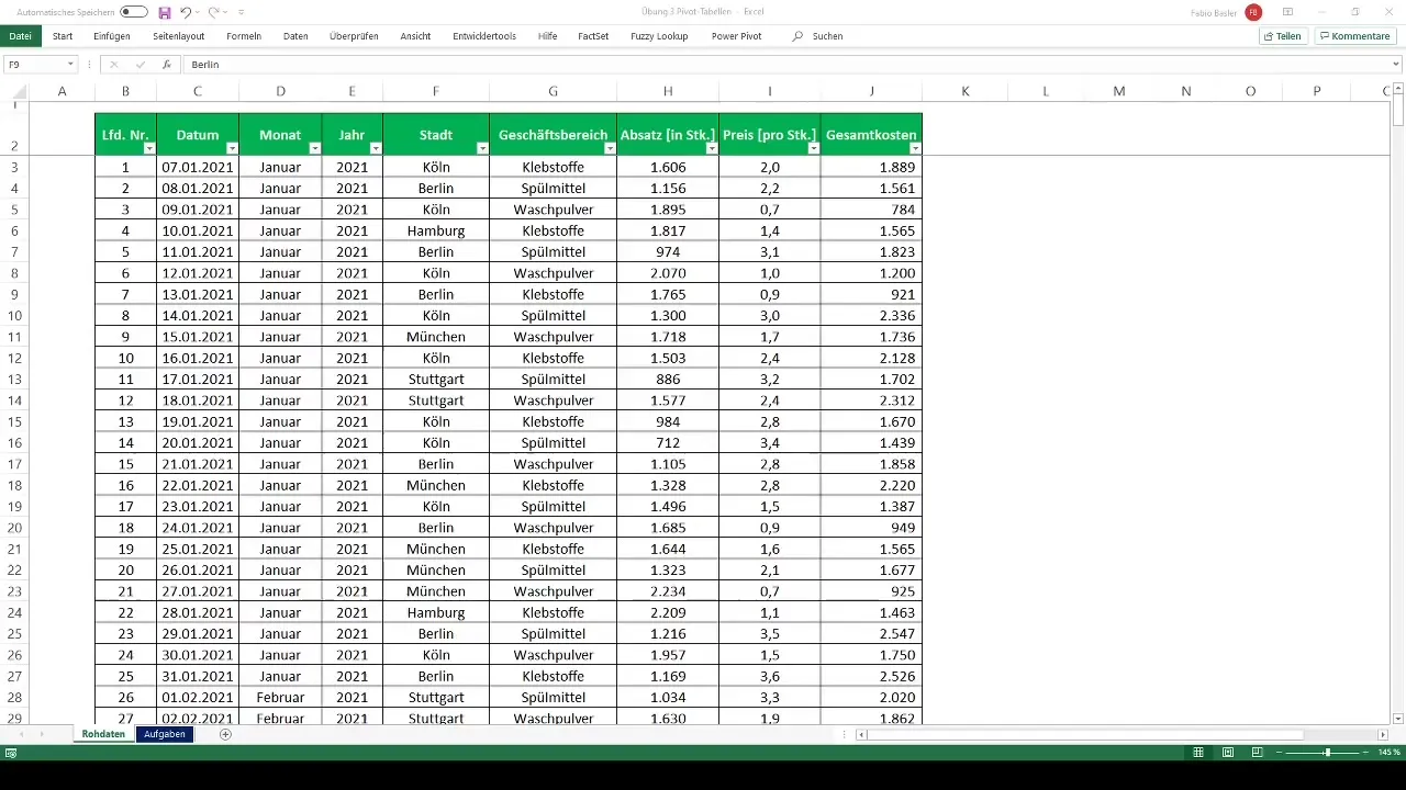
To start your analysis, you must first access the provided dataset. In this case, it consists of sales figures of a consumer goods company active in the adhesive, detergent, and laundry detergent sectors. You should keep an eye on data such as sales figures, prices, and total costs.

Now it's time to create the pivot table. Select the entire range of data and go to the "Insert" tab in Excel. Choose "PivotTable". In the subsequent dialog, you can set the location of the table - whether in a new worksheet or in the existing one. Confirm your selection, and you will have an empty pivot table in Excel.

Step 2: Drag Data Fields into the Pivot Table

Once the pivot table is ready, you can start dragging relevant data. Drag the cities (e.g., Berlin, Hamburg, Cologne, Munich, Stuttgart) into the rows field of the pivot table and the business areas (adhesives, detergents, laundry detergent) into the columns field. Then drag the sales and price data into the value field to generate an initial overview of the sales figures.

Step 3: Calculate Revenue and Profit

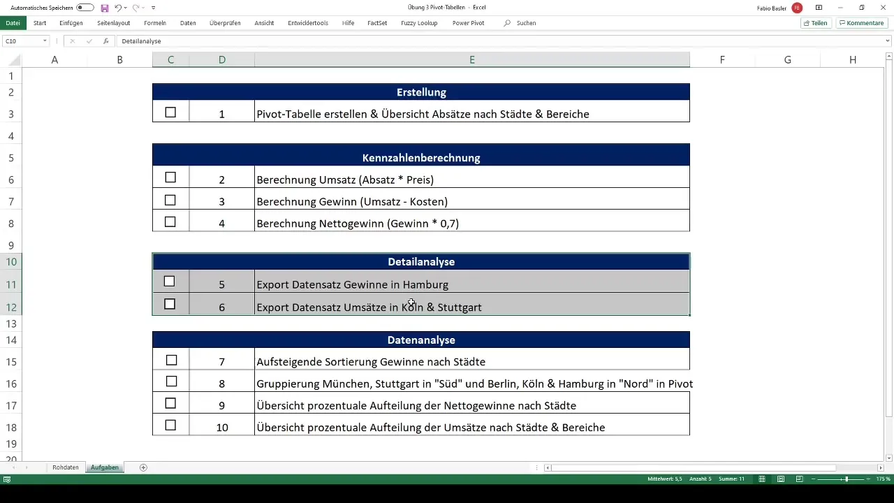
After creating the initial overview, you can now start calculating key figures. To determine revenue, multiply the sales figures by the prices. Add a new column in the pivot table representing revenue.

To calculate profit, subtract the total costs from the calculated revenue. Here too, you can add a new column in the pivot table to visualize the profit.

Step 4: Calculate Net Profit after Tax Rate

In the next step, you will calculate the net profit by subtracting 30% from the profit. In Excel, you can easily do this by entering the appropriate formula in the column for net profit:

Net Profit = Profit * (1 - Tax Rate)

Set the tax rate to 0.3 to determine the net profit.

Step 5: Perform Detailed Analysis

Now that you have the key figures, it's time for a detailed analysis. You should export data from specific cities, such as Hamburg. You can achieve this by double-clicking on the pivot cell with the relevant data. This will give you a new table listing the information specific to that city.

Step 6: Perform Ascending Profit Sorting and Grouping

Now we move on to more complex analyses. To better structure your data, you can sort profits by cities in ascending order. Right-click on the profit column and select "Sort".

Additionally, you can group cities: for example, place Munich and Stuttgart in the "South" group and the cities Berlin, Cologne, and Hamburg in the "North" group. This facilitates a comparative analysis between the groups.

Step 7: Create Percentage Allocation in Pivot Overview

In this final step, we will create a percentage allocation for net profits. You can do this by creating a new pivot table based on the data already created. Add the cities and their respective net profits to your new pivot table and select the option for percentage representations.

Enjoy implementing each task! It's a good idea to work through everything step by step and refer back to the content of the previous lessons if needed.

Summary

This tutorial has shown you how to effectively work with pivot tables in Excel. From creating the table to calculating key figures to detailed analyses, you have learned important steps that will help you evaluate data comprehensibly and systematically.