Your goal is to analyze data in a way that is not only precise but also straightforward. Pivot tables in Excel give you the opportunity to effectively manage and present large datasets. In this guide, you will learn how to perform a detailed analysis of your pivot tables through simple clicks. This step-by-step guide will help you maximize the full potential of your data.
Key Insights
- You can generate detail reports by double-clicking on cells in pivot tables.
- Using slicers helps filter data for specific information.
- It is possible to create new pivot tables from filtered data to conduct even more targeted analyses.
Step-by-Step Guide
To use your pivot tables for detailed analysis, follow these steps.
1. Creating the Pivot Table
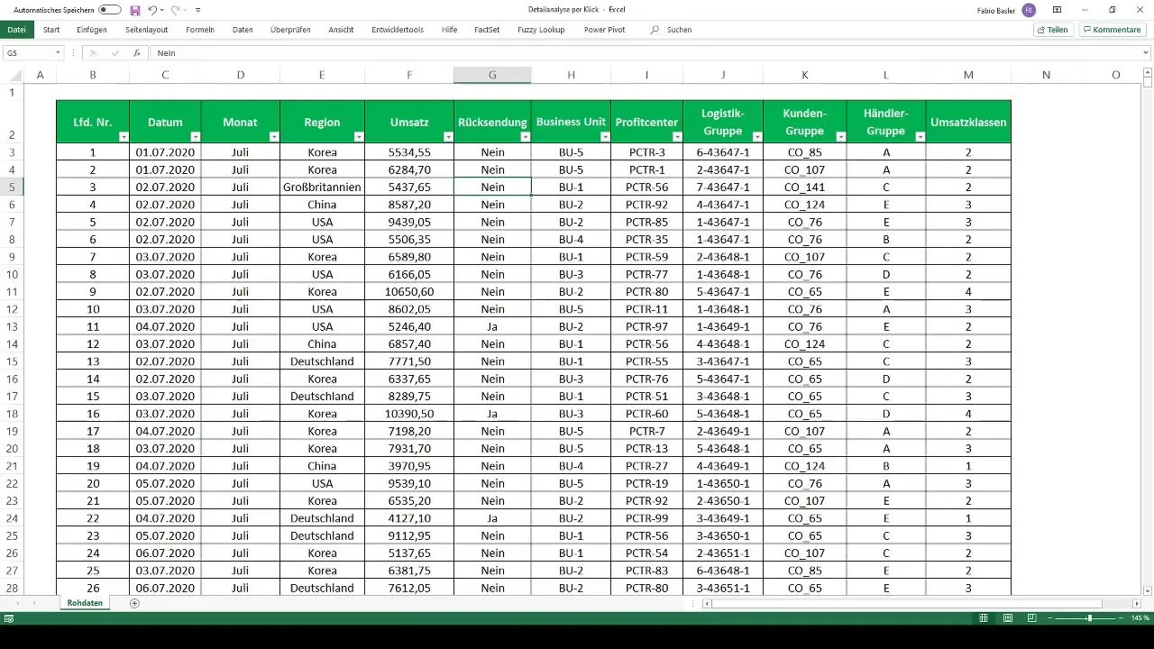
First, ensure that your source data in Excel is well-structured. Begin by selecting your data and creating a table with the Ctrl + T keyboard shortcut. Then go to "Insert" and select "PivotTable". A new worksheet will open for the pivot table.
2. Adding Values
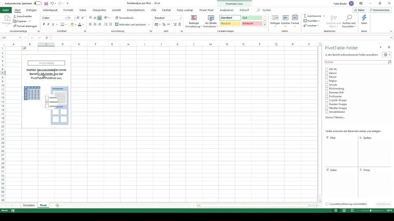
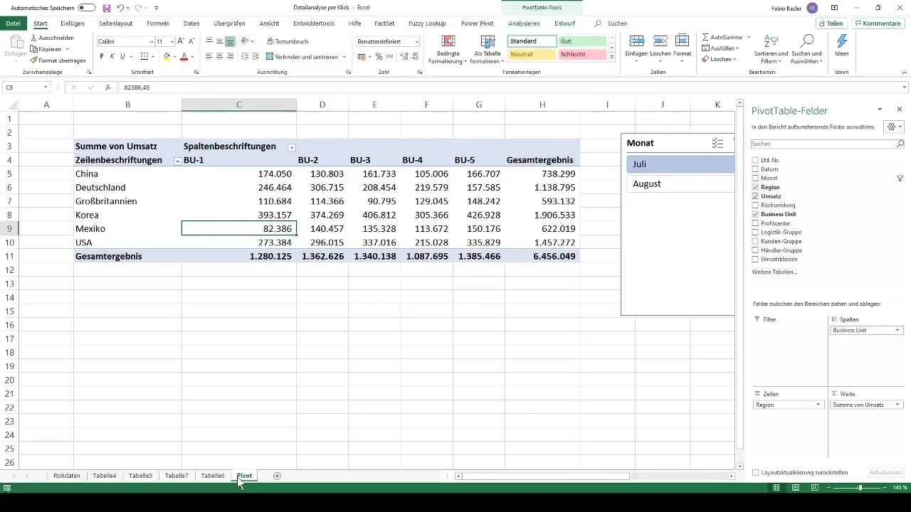
Now is the time to add your values. Drag the revenue amount into the value area of your pivot table. To conduct a meaningful analysis, also drag the various business units and regions into the column or row fields.
3. Using Slicers
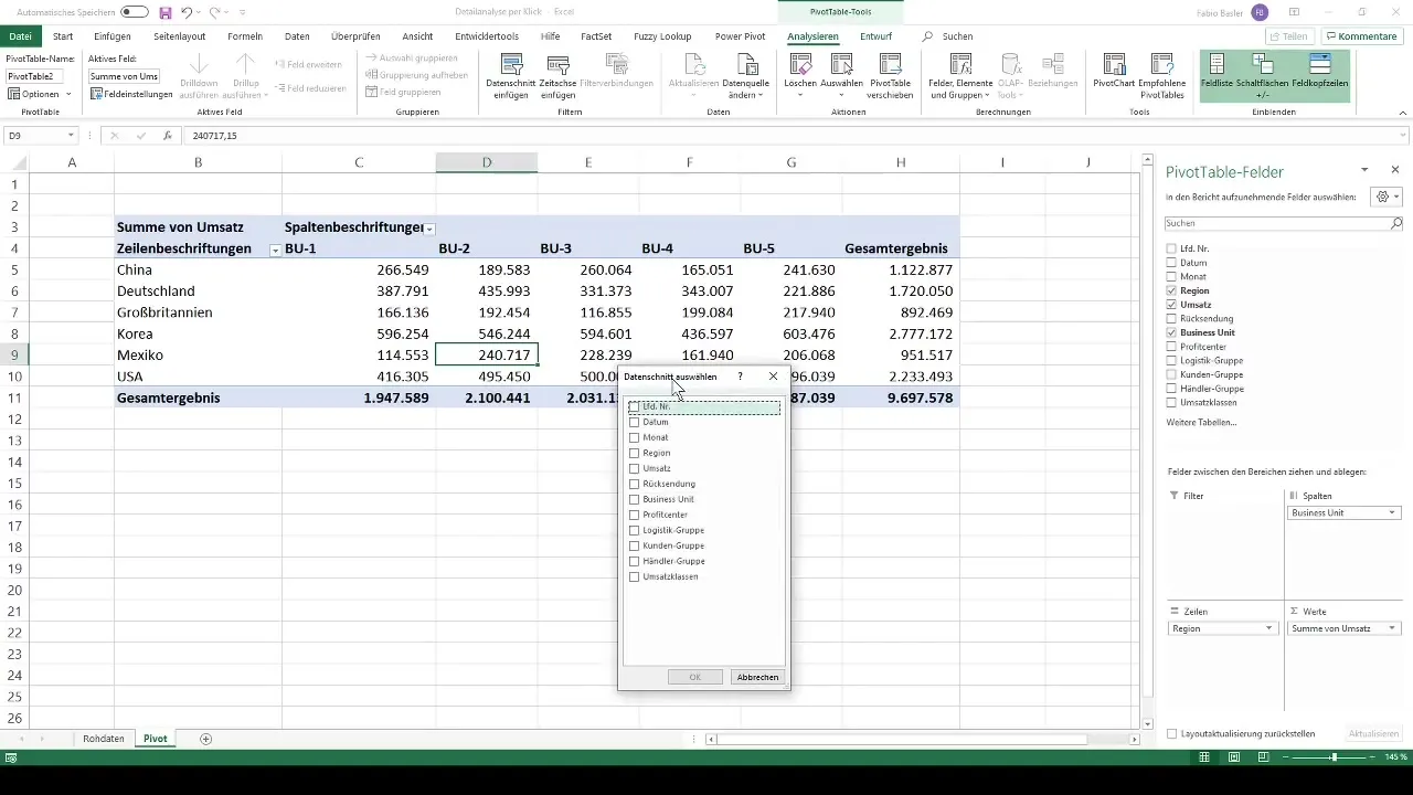
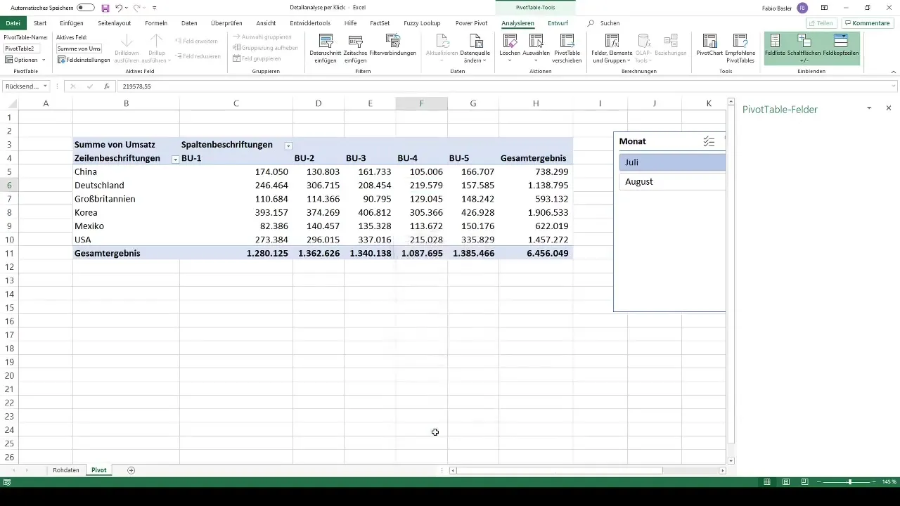
To further refine your analysis, you can add slicers. These help you create specific reports based on time periods or specific business areas. Click on "PivotTable Analyze" and add a slicer for months. This provides a filtering option to analyze a specific time period.
4. Granular Data View with Double-Click
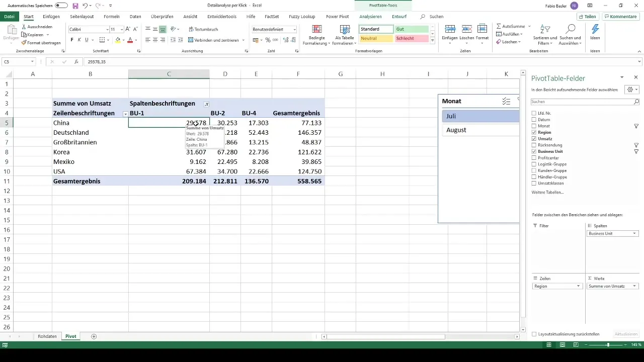
A particularly powerful tool in pivot tables is the ability to generate specific detail reports by double-clicking on a number. For instance, if you want to see the revenue for a specific region and month, double-click on the revenue value. Excel will automatically create a new table with the underlying data.
5. Filtering Results
If you want to make further specifications, you can use additional slicers. These allow you to filter data by business units or returns. Go back to your PivotTables tools and select "Add Slicer". Specify the criteria you want to filter by.
6. Aggregation in New Pivot Tables
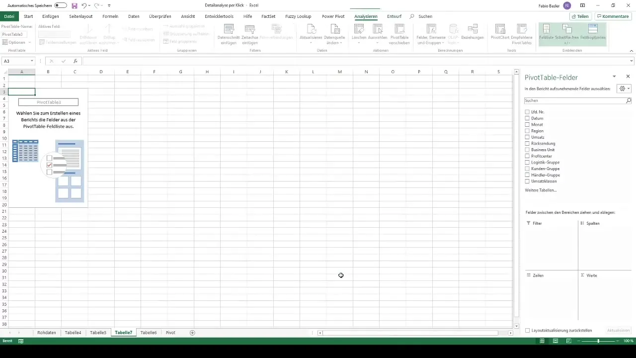
After the detailed analysis, it can be helpful to summarize the filtered information in a new pivot table. Click on the aggregated data and select "Create PivotTable". This allows you to generate a new report containing only the data you selected.
7. Sharing Analyses
Finally, it is common to share the results with your colleagues or other departments. Exporting to Excel or CSV format is easily possible. You can also send the new pivot table directly to colleagues who are only interested in those specific data.
Summary
By following the steps described above, you are well-equipped to conduct effective detailed analyses with pivot tables in Excel. Utilize the capabilities to quickly filter specific information and create understandable reports. From data aggregation to solving complex questions: With these techniques, you can revolutionize your data analyses.
Frequently Asked Questions
How do I create a pivot table?Select your data, go to "Insert," and click on "PivotTable."
How can I add a slicer?Go to "PivotTable Analyze" and select "Insert Slicer."
What happens when I double-click on a pivot cell?Excel automatically creates a new table with the details of the underlying data.
Can I aggregate filtered data in a new pivot table?Yes, you can easily transfer filtered data to a new pivot table.
How can I best share my pivot analyses?Export the pivot table to an Excel or CSV format or send the table directly to interested colleagues.


