How to calculate percentage values in pivot tables

You want to understand how you can effectively perform percentage calculations in Pivot Tables in Excel? This guide will take you through a clearly structured process to make the wealth of information in your data visible. In particular, we will show you how to create and interpret percentage figures in relation to subcategories. Through a practical example, you will learn step by step how to work with the various functions of Excel.

Key Insights

• Percentage values can be calculated both from the total result and from subcategories.
• You can integrate various dimensions into your Pivot Table to gain different perspectives.
• Adjusting the reference size enables deeper insights into the underlying data.

Step-by-Step Guide

Format data for Pivot Table

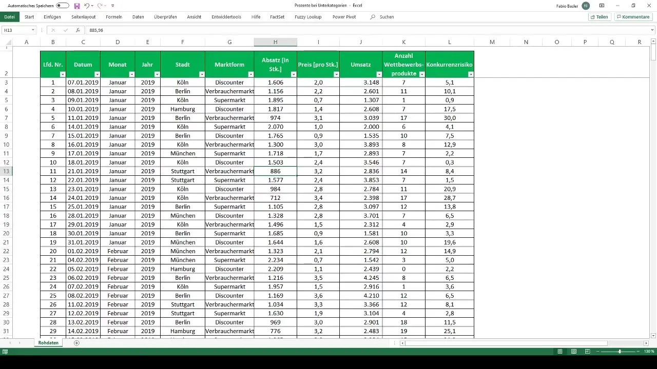
To start analyzing your data, it is necessary to select your entire data range and format it as a table. You can efficiently do this by pressing Ctrl + T. This will provide you with a solid foundation for your subsequent calculations.

Create Pivot Table

After formatting your data as a table, you can create the Pivot Table. Go to the ribbon menu and select the options to create a Pivot Table. Choose the range of your formatted table and create the Pivot Table on a new worksheet.

Analyze revenues and present them as percentages

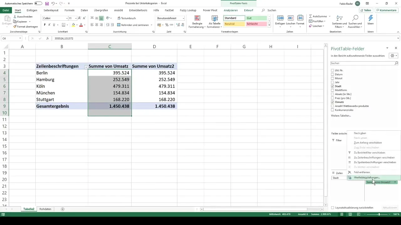
Now that your Pivot Table is created, you have access to the individual data fields. You can now analyze revenues by cities. Drag the revenue field into the data area of your Pivot Table. This will provide you with the absolute numbers for revenue in each city.

Show values as percentages

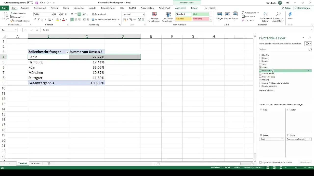
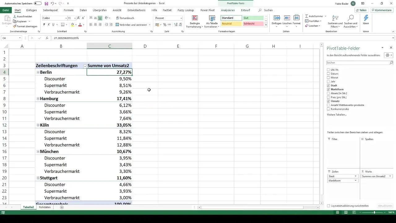
To convert the absolute revenue representation into percentage values, right-click on the revenue field in your Pivot Table and select "Value Field Settings". Under the settings, you can now choose the option "Show values as" and select "Percentage of Grand Total". This will show you how much each part contributes to the total revenue.

Incorporate additional dimensions

For deeper analyses, you can add additional dimensions to your Pivot Table. Also, drag the market type field into the columns. This allows for a detailed analysis by various distribution channels – such as discounters, supermarkets, and consumer markets.

Adjust reference size

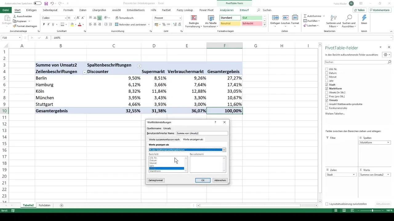
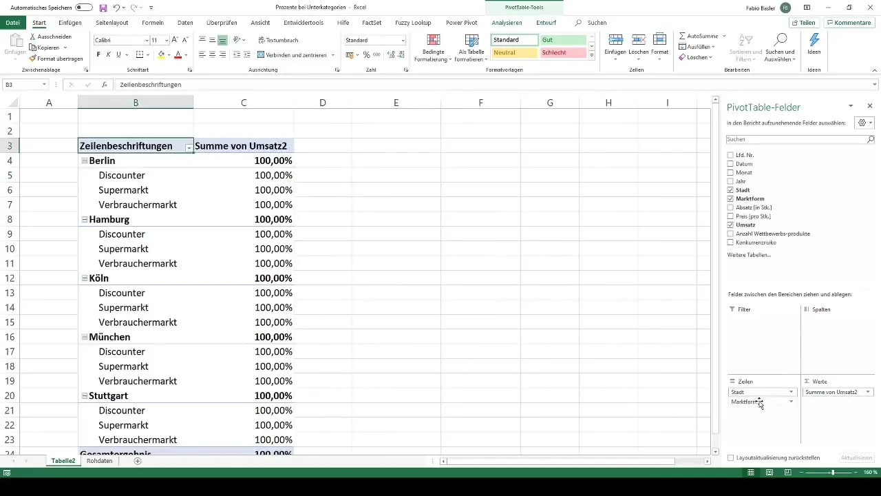
To refer calculations to a specific market type or city, you can adjust the reference size. Go back to "Value Field Settings" and this time select "Percentage of" along with the appropriate dimension you want to use as a basis. This will display the revenue for each market as 100%, and the percentage values for individual cities will be calculated relative to this base value.

Show percentage breakdown of individual markets

If you now want to break down sales by market type, you can drag the "Market Type" field into the column header while leaving the revenue field in the data area. This will give you an insight into the percentage distribution of revenue across the various market types. You will see that the respective percentages vary due to the shifted perspective.

Alternative calculation methods

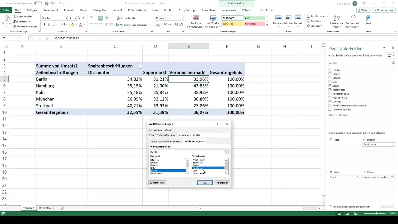
Excel also offers the option to select specific base values for percentages. For example, you can specify that the revenues should be calculated relative to a single city, such as Hamburg. Simply set the reference size accordingly to make these adjustments.

Graphical representation of results

To visually present your results, you can create diagrams or graphics. This not only helps to illustrate the data, but also facilitates the communication of the results to team members or executives.

Summary

In this guide, you have learned how to effectively perform percentage calculations within Pivot Tables in Excel. You have learned how to calculate both from the total result and from subcategories, and what customization options Excel provides you.