Create your first pivot table in Excel

Equipped with Pivot Tables, any data analyst can generate impressive insights from large data sets. These tables provide a dynamic method for organizing, analyzing, and visualizing data. In this guide, you will learn how to successfully create and model your first pivot table in Excel to extract valuable information from your data.

Key Insights

• Pivot tables enable flexible data analysis and visualization.
• You can utilize multiple dimensions to conduct complex evaluations.
• You can customize the representation of your data according to your needs.

Step-by-Step Guide

Understanding the Basics of Pivot Tables

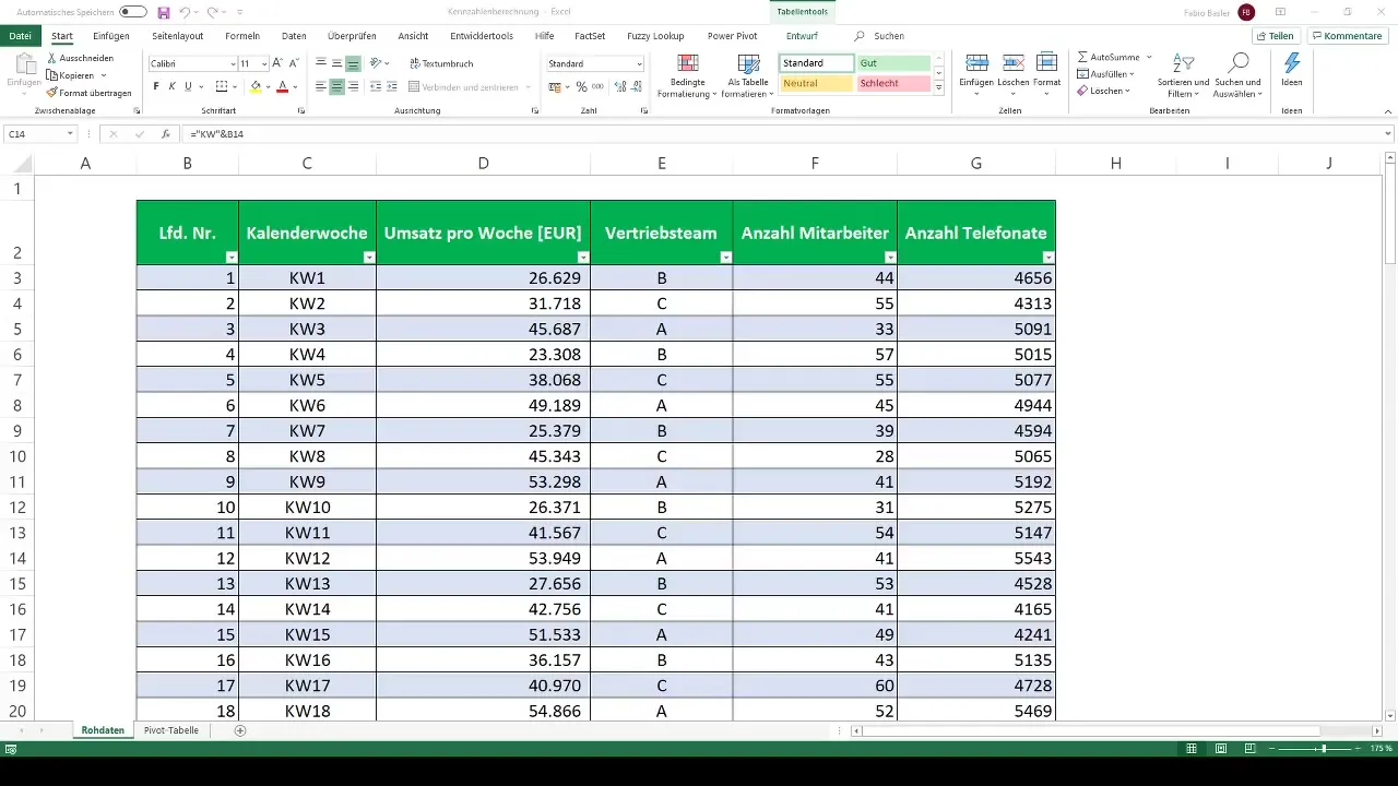
Before you begin creating the pivot table, it's important to understand how your data should be structured. Ensure that your raw data set is clear and organized. A well-structured data foundation requires consistent column headings and no empty rows.

Creating Your First Pivot Table

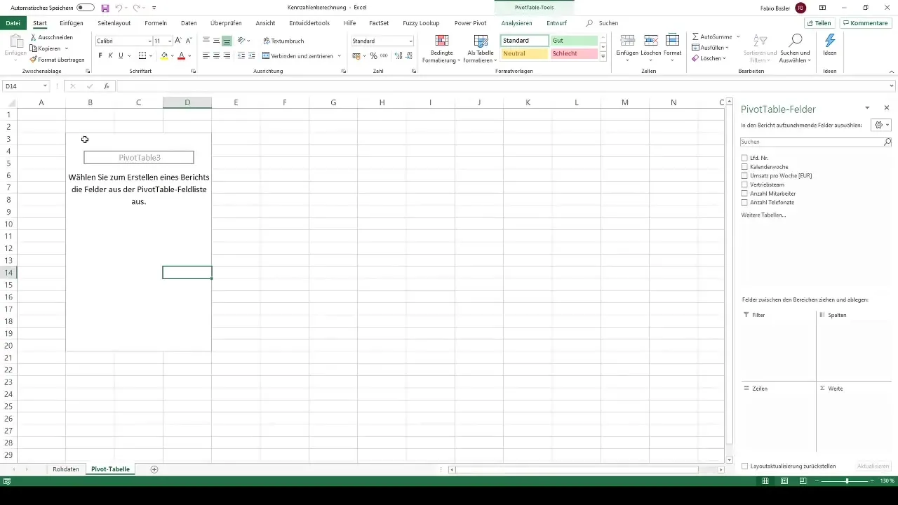
Now let's jump straight to the practical example. You have already created an empty pivot table in Excel that has not been populated yet. To start working, you need to activate the PivotTable fields. Click in the pivot table area for the fields to become visible on the right side. These fields display all available dimensions of your data.

Assigning Dimensions

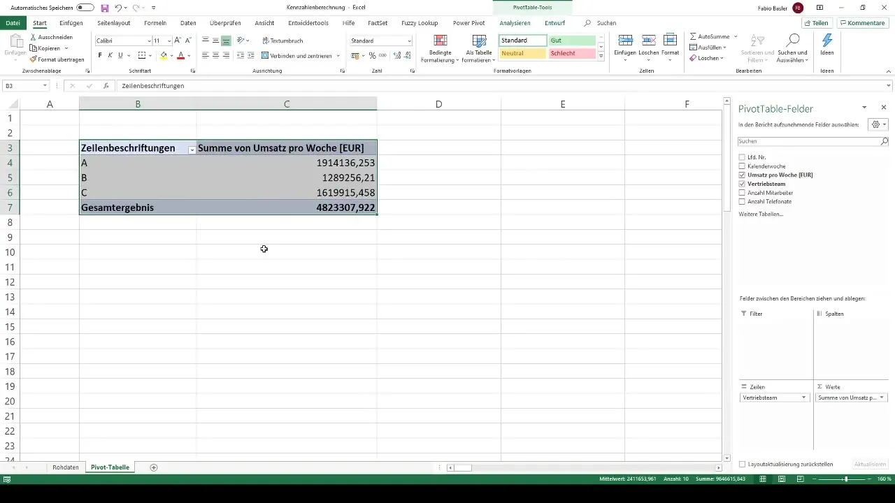
To effectively populate your pivot table, you can use various dimensions such as filters, columns, rows, and values. Firstly, drag a metric from the list into the value field. Let's say you want to analyze revenue. Check the revenue field, and it will automatically be integrated into the value field of your pivot table.

Adjusting Data Models

Now for the exciting part: dynamically modeling your pivot table. You can add different metrics at any time. For example, drag the sales feature into the rows. This creates your first two-dimensional structure – the basic form of your pivot table.

Changing Structure

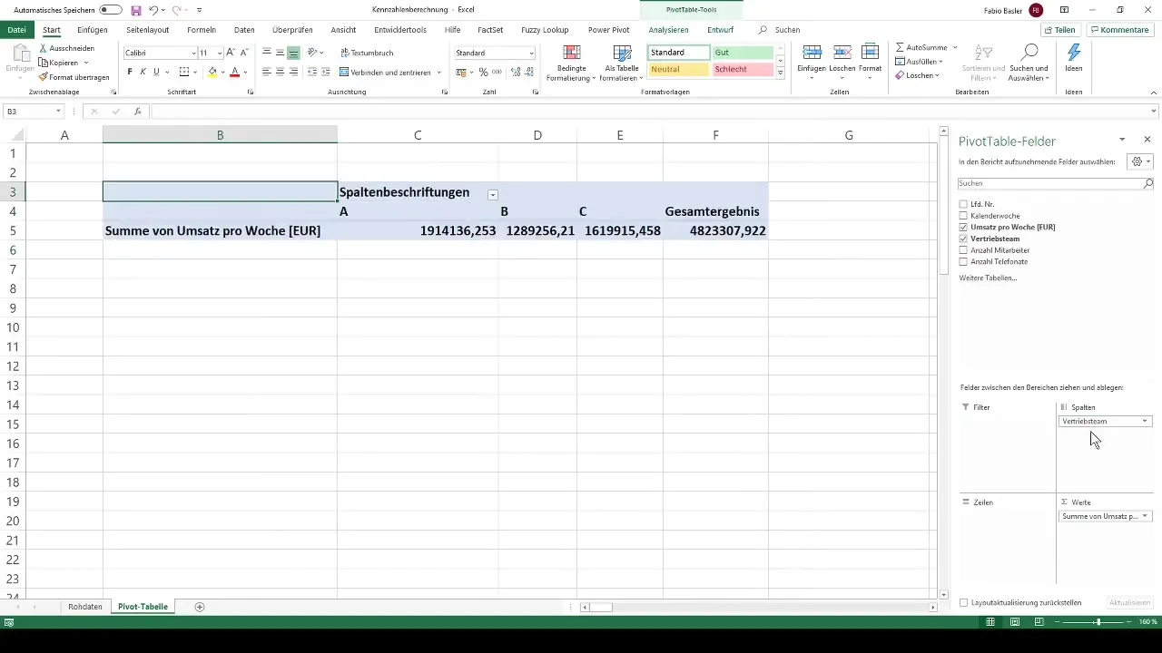
One of the strengths of pivot tables is the ability to easily alter the structure of your data. For instance, you can switch the row and column arrangements. Experiment with arranging your dimensions to gain different perspectives on your data. Drag the sales feature into the columns and observe how the representation changes.

Utilizing Filters

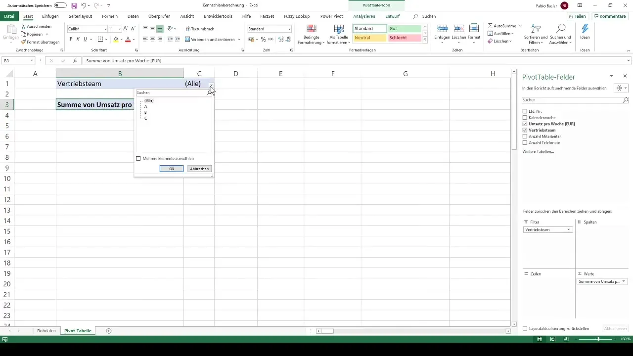
To further refine the pivot table, you can also implement filters. Drag the sales team into the filter area to display specific sales areas only. For example, you can show data only for sales teams A and B while excluding data for team C.

Reviewing Results

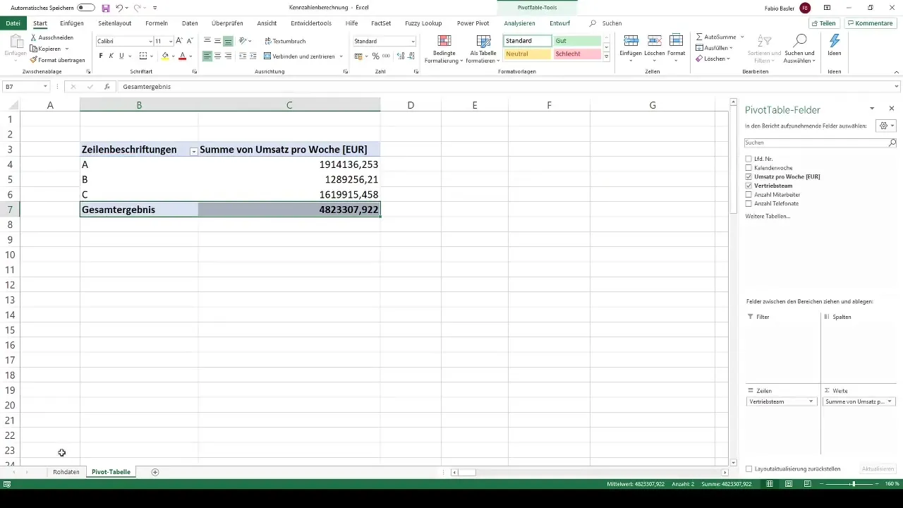
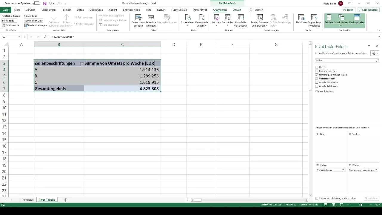
After adjusting the structure of your pivot table, you can identify the revenue distribution for each team. You will see the respective revenue figures and the consolidated revenue across the analyzed period.

Data Formatting

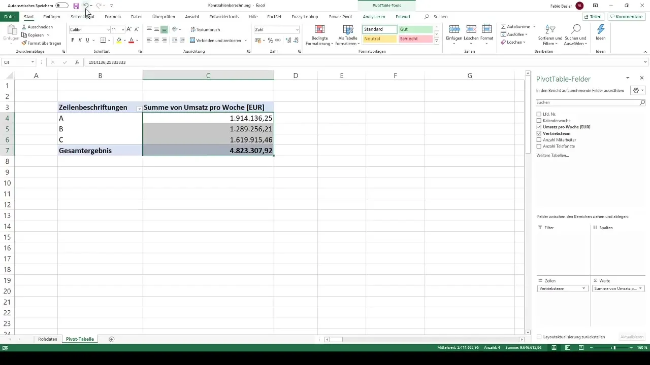
The numbers in your pivot table may not be optimally formatted yet. To ensure that the values are clear and easy to understand, apply formatting for thousands. Use the keyboard shortcut Ctrl + Shift + 1 to add the thousand separator or click on the corresponding symbol in the toolbar.

Making Adjustments

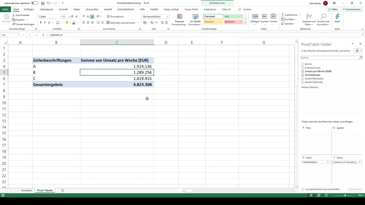
You can also adjust the number of decimal places. Remove the decimal places to make the data even clearer. After these adjustments, the revenue for the respective sales teams will be displayed clearly and distinctly.

Outlook on further functions

You have now successfully created and modeled your first pivot table. In the next lessons, we will focus on additional ways for you to select and display more complex evaluations and calculations, including averages or other metrics, in your pivot table.

Summary

You have now learned how to create a pivot table in Excel, adjust its dimensions, and effectively format the data. With these skills, you'll be able to gain valuable insights from extensive data sets and present them in a visually appealing way.