Key figure calculation in Excel pivot tables

You want to effectively use pivot tables in Excel? Calculating key figures is a central part of obtaining valuable and meaningful information from raw data. In this guide, you will learn how to calculate and visualize various metrics in a pivot table. We will go through the basic steps to obtain sum, average, maximum, minimum, and standard deviation. Additionally, we will show you how to represent percentages of total results.

Main Insights

• Pivot tables enable easy calculation of metrics.
• You can calculate sums, averages, maximum, minimum, and standard deviation.
• It is possible to represent metrics as percentages.

Step-by-Step Guide

1. First Contact with the Pivot Table

To start with calculating key figures, open your pivot table in Excel. You will notice that clicking on the pivot table reveals a ribbon with various options on the right side. The menu helps you to make the necessary calculations and select the desired representation.

2. First Metric: Sum

Upon opening the pivot table, you will already see that a first metric - the sum - has been automatically calculated. This standard calculation shows you the entirety of your data.

3. Accessing Value Field Settings

Click on the sum in the pivot table. On the right, the "Value Field Settings" field opens. Alternatively, you can also navigate through the ribbon above to access the fields. Here, you have the option to select various calculation methods.

4. Calculating Average Values

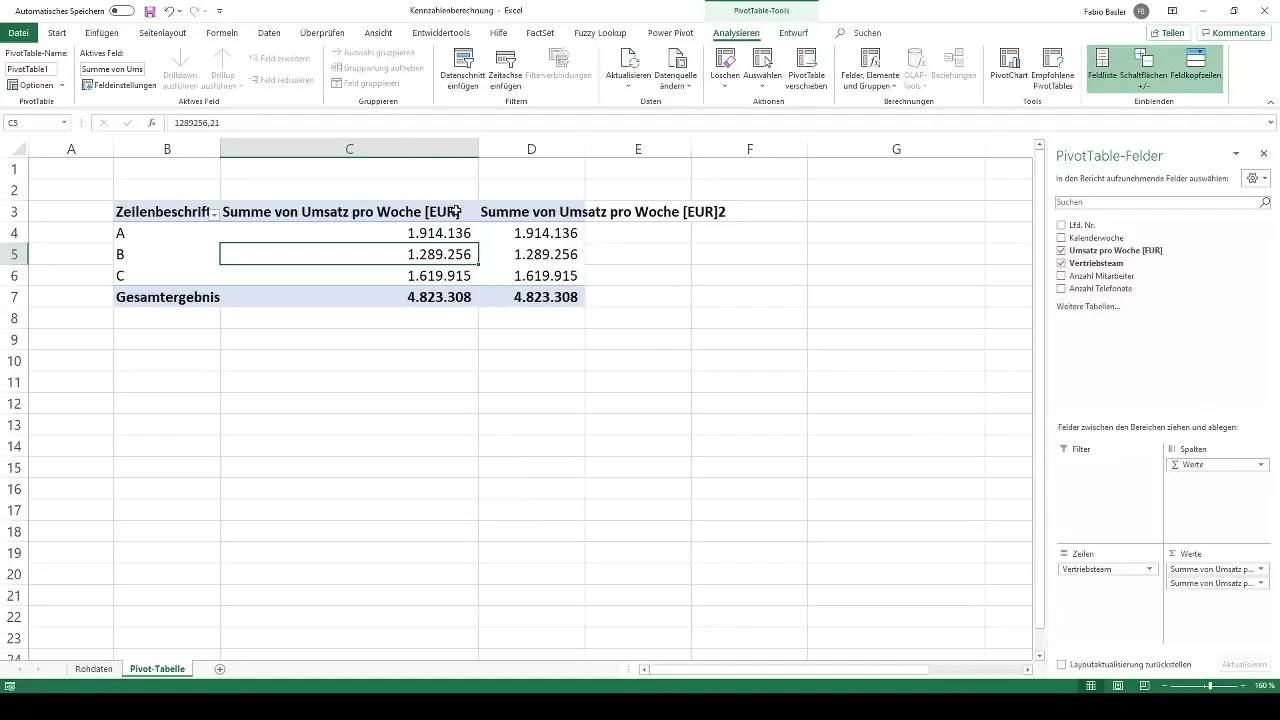
Now you can, for example, drag the revenue per week into the value area of the pivot table. You will see that a sum is also displayed. To calculate an average, go back to the value field settings and change the function from "Sum" to "Average".

5. Insights into Average Values

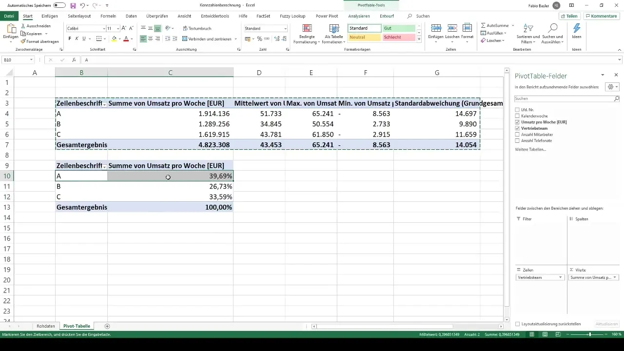
Now, you will see both the consolidated revenues per sales team and the average values per week. For example, it looks like sales team A achieved an average revenue of about 51,000 euros, while B and C are around 35,000 and 43,000 euros, respectively.

6. Deepening the Metrics

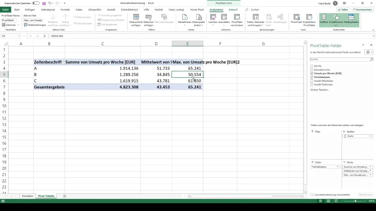
Now you can add more metrics. Drag the revenue back into the pivot table and change the setting in the value field settings. In addition to average and count, you can also calculate the maximum. This is selected through the "Maximum" option in the same menu field.

7. Minimum and Standard Deviation

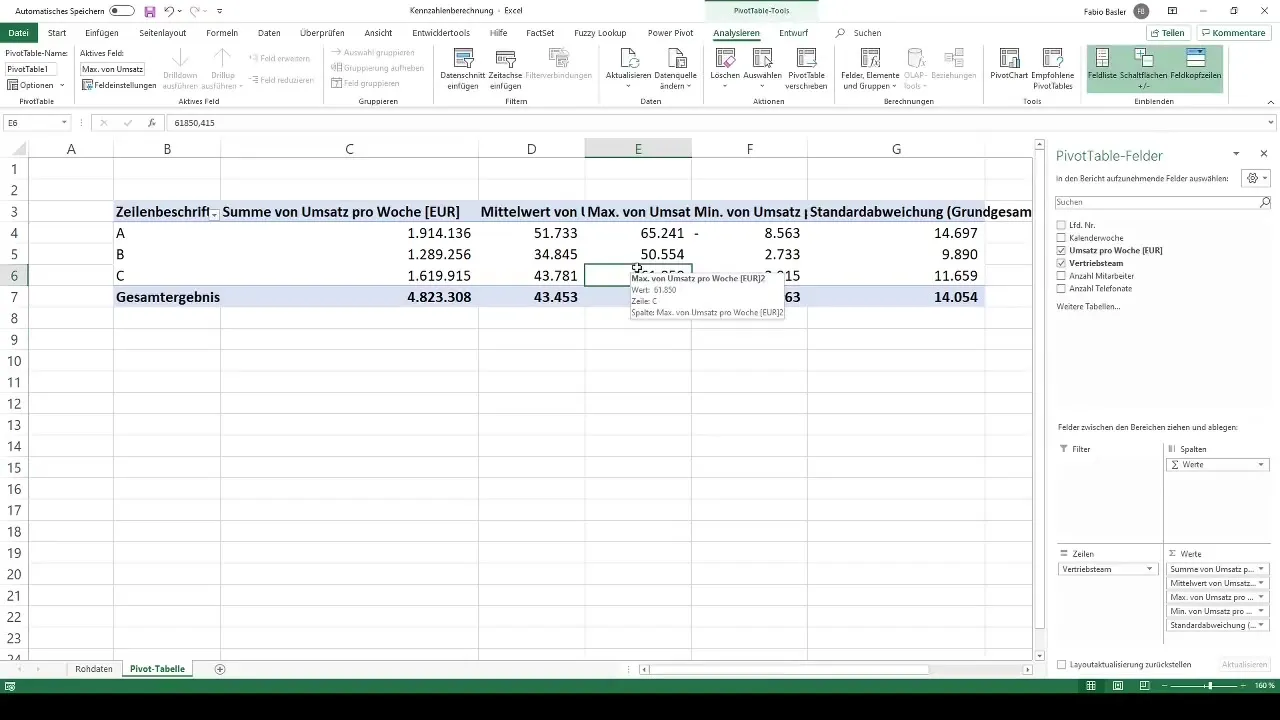
For a more comprehensive analysis, drag the revenue into the table once again. Now you can also calculate the minimum, for example. Furthermore, you can also add the standard deviation to analyze the fluctuations in your revenue per sales team.

8. Understanding Standard Deviation

The standard deviation provides information about the variations in your revenue values over the weeks. It is calculated by squaring the differences from the mean. These sums are then divided by the number of values to further quantify the deviations.

9. Adding Advanced Metrics

With this, you have already calculated five important metrics in your pivot table. In future lessons, you will learn how to add individual metrics using the "calculated field" option. This allows you to calculate additional KPIs based on existing fields.

10. Representing Percentages

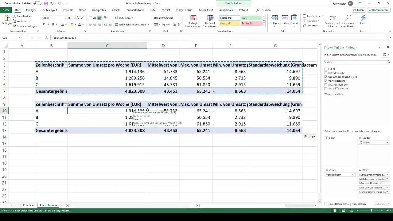
To have a percentage view of your data, you could also copy your pivot table. Now you have the option to represent the sum not only as an absolute value but also as a percentage of the total result. You can use the various display options for percentages in the menu.

11. Conclusion of Sales Performance

In the final pivot table, you have the opportunity to display the sales performance per sales team in percentage. For example, you can see that sales team A accounts for 39% of the total sales, B 26%, and C 33%.

Summary

Calculating metrics in pivot tables is an important step to effectively analyze your data. You can perform complex analyses from simple sums - from averages to maximum and minimum values to standard deviation. With these valuable insights, you are able to thoroughly evaluate your data and substantiate presentations precisely.