Excel offers a powerful way to analyze large amounts of data with Pivot Tables. But what if the underlying data changes or expands? In this guide, I'll explain how you can change the data source of a Pivot Table in Excel. With a few simple steps, you can keep your analysis up to date and efficient.
Key Takeaways
- The data source of a Pivot Table can be changed using the menu bar.
- It is advantageous to format the data as a table to keep the reference ranges flexible.
- Changing the data source helps ensure the accuracy of the analyses, especially with changing data.
Step-by-Step Guide to Changing the Data Source
To customize your Pivot Table, follow these steps. First, make sure you are working with the current database.
Step 1: Check the Current Data Source
If you have already created a Pivot Table, you can view the current data source. Click on the Pivot Table to do so.
Step 2: Accept Changes in the Data Source
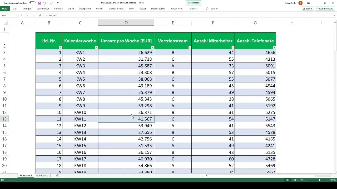
Return to your raw data set to see if new data has been added or the structure has changed. If you find that the range has been expanded, you need to make this adjustment in the Pivot Table.
Step 3: Change Data Source in the Menu Bar
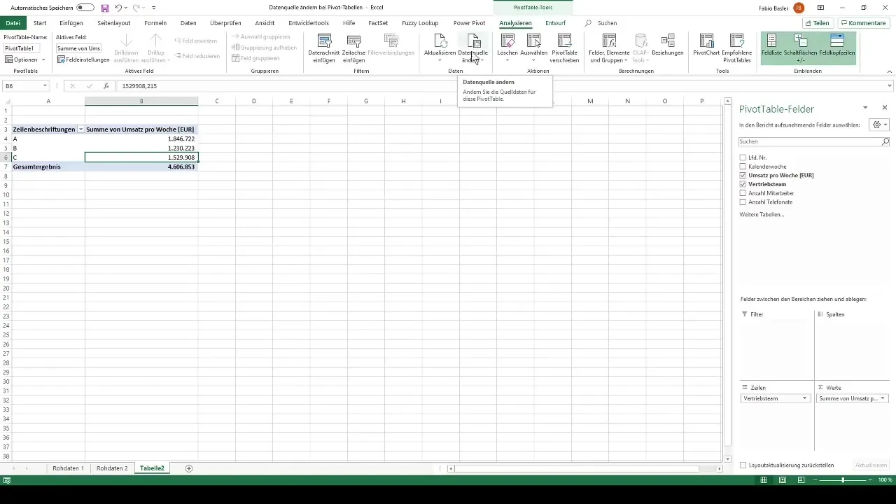
Go to the menu bar and click on "PivotTable Tools." There you will find the option "Change Data Source." Click on it to modify the data source.
Step 4: Modify the Source Data
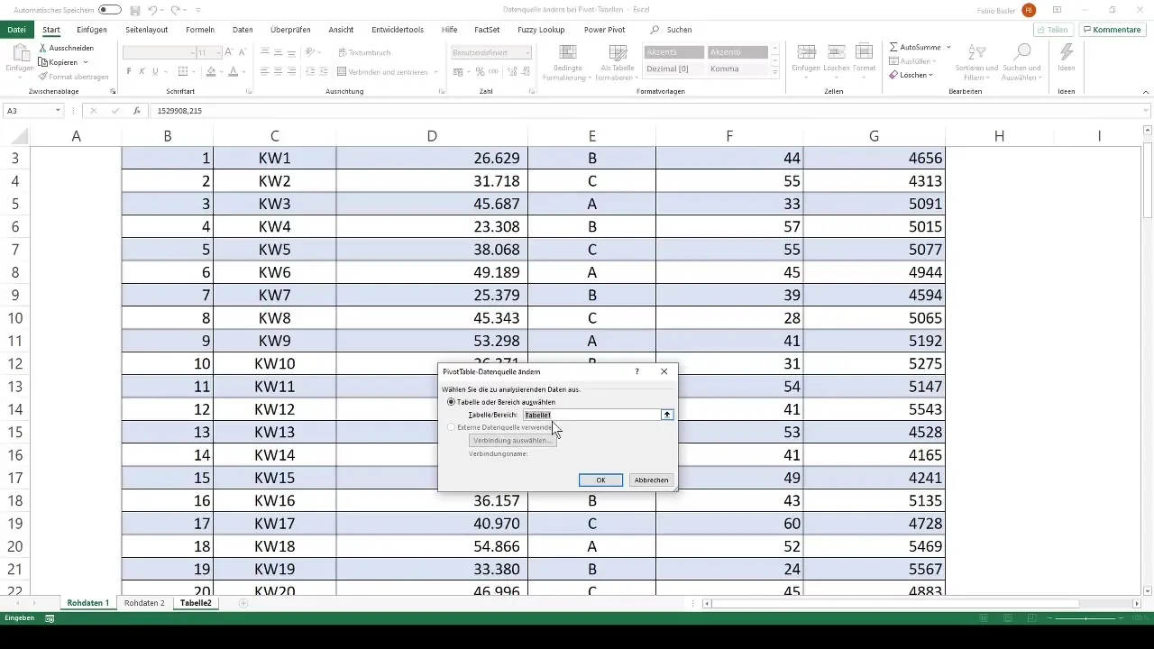
If your data has been formatted as a table, you will only see the reference as "Table 1." Otherwise, you will need to manually specify where the new data can be found.
Step 5: Select the New Data Source
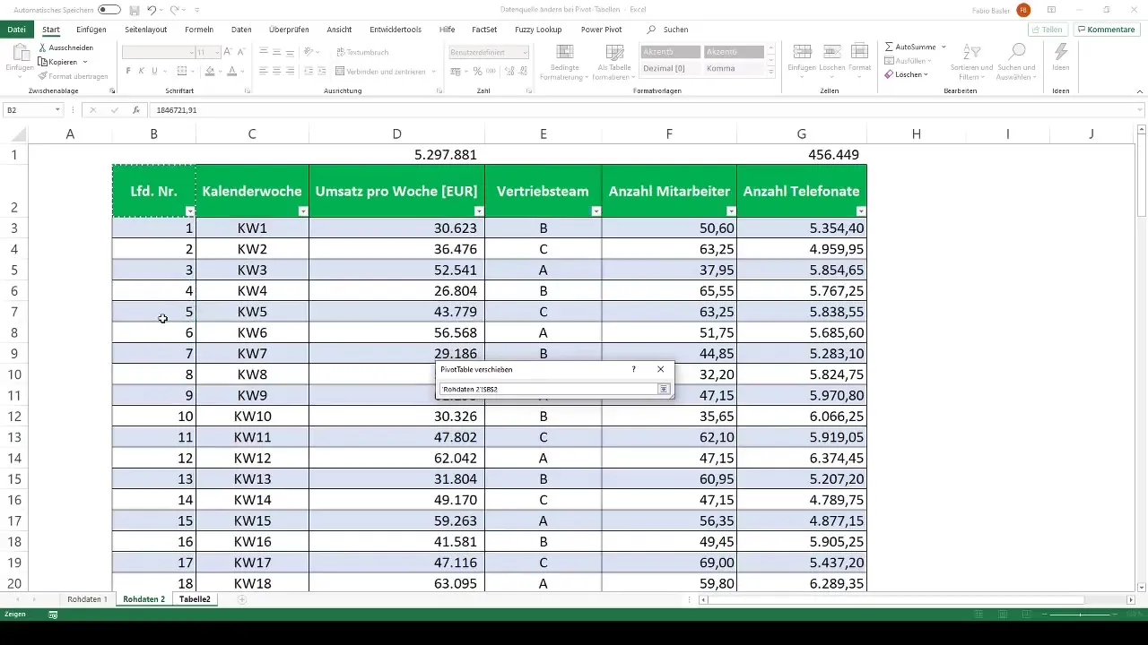
Now you should select the new data source. For example, if you already have a table with new data whose name you know, select that table accordingly.
Step 6: Update the Pivot Table
After changing the data source, go back to your Pivot Table and refresh it. Simply click on the "Refresh" button in the "PivotTable Tools." This ensures that the latest data appears in your analyses.
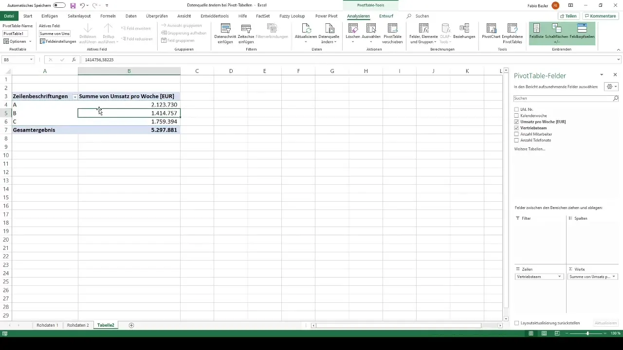
Step 7: Review the Updated Values
Finally, review the updated Pivot Table. Check if the new values are calculated correctly to ensure the accuracy of your analyses.
Summary
By changing the data source of your Pivot Tables, you can ensure that your analyses are always based on the latest information. It's important to format the data as a table to optimize the process. With these simple steps, you can quickly respond to new data and effectively keep your analyses flexible yet efficient.
Frequently Asked Questions
How do I change the data source of a Pivot Table?Go to "PivotTable Tools" and click on "Change Data Source" and select the new data source.
Why should I format my data as a table?Formatting data as a table allows the reference to automatically expand when new data is added.
Can I manually enter the data source?Yes, you can manually define the data source by specifying the cell range.
Do I need to refresh the Pivot Table after changing the data source?Yes, you need to refresh the Pivot Table to display the latest data.


