Learn how to create a pivot table in Excel

Pivot tables are a powerful tool in Excel that helps you analyze and present data effectively. In this guide, I'll show you step by step how to create your first pivot table. Understanding the structure and the data you want to analyze is crucial to fully utilize the benefits of pivot tables.

Key Insights

• Data must be in a structured format.
• You can create pivot tables directly from a selected data range.
• When selecting the pivot table data source, it is important to consider future data changes.
• Formatting your raw data as a table helps to dynamically adjust the data source.

Step 1: Data Preparation

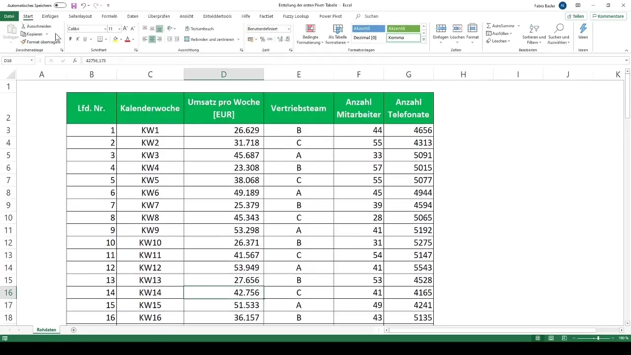
Before you start creating your first pivot table, it is important that your data is in a clear and structured format. Ensure that all data is consistently arranged and does not contain any empty rows or columns.

Step 2: Open Ribbon and Select Pivot Table

To start creating your pivot table, you need to open Excel's ribbon bar. Simply press the "Ctrl" and "F1" buttons.

Then navigate to the "Insert" tab and click on the "Pivot Table" button. This is the first step towards generating your analysis.

Step 3: Select Data for Pivot Table

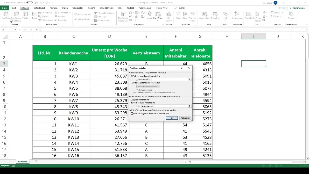
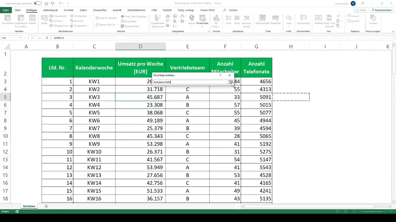
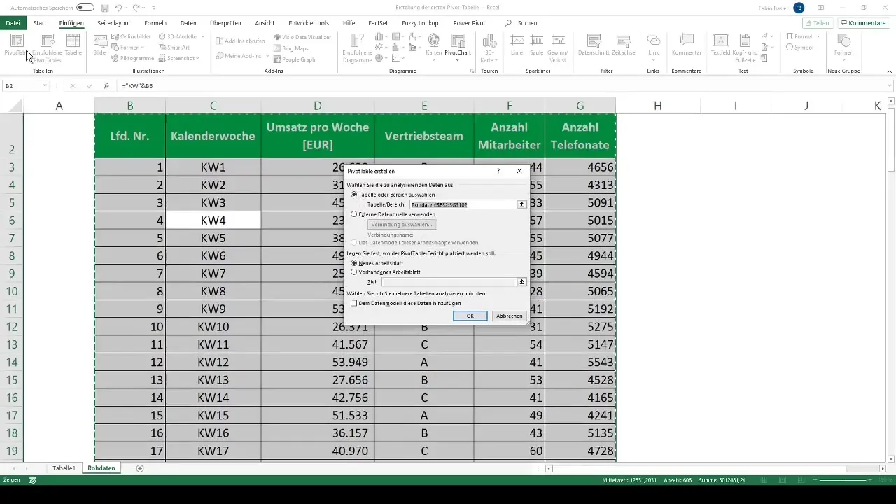
After clicking on "Pivot Table," the entire data range serving as input will be automatically displayed. It's important to ensure that this data range is correctly selected. If you click outside the data range, you will need to manually specify the range.

Here, make sure to include cell references to ensure that the pivot table can update independently of future changes to the data.

Step 4: Define Pivot Table Position

Now you have the option to define the position for your pivot table. There are two options:

1. Create a new worksheet.
2. Insert the pivot table into an existing worksheet.

For clarity, I recommend using a new worksheet. This makes it easier to separate raw data from pivot analysis.

Step 5: Finalize Pivot Table

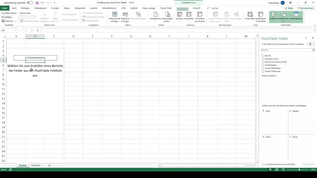
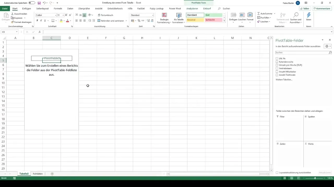
After setting the input data and position, click on "OK." Your first pivot table is now created. It is named "Pivot Table 1" by default.

Step 6: Using Shortcuts for Simplification

To streamline the creation of your pivot tables, you can use various shortcuts. You can quickly select the entire data range by pressing "Ctrl + A." This saves time, especially when working with large datasets.

Alternatively, you can manually highlight the range you wish to analyze before clicking on the pivot table.

Step 7: Setting Up Dynamic Data Source

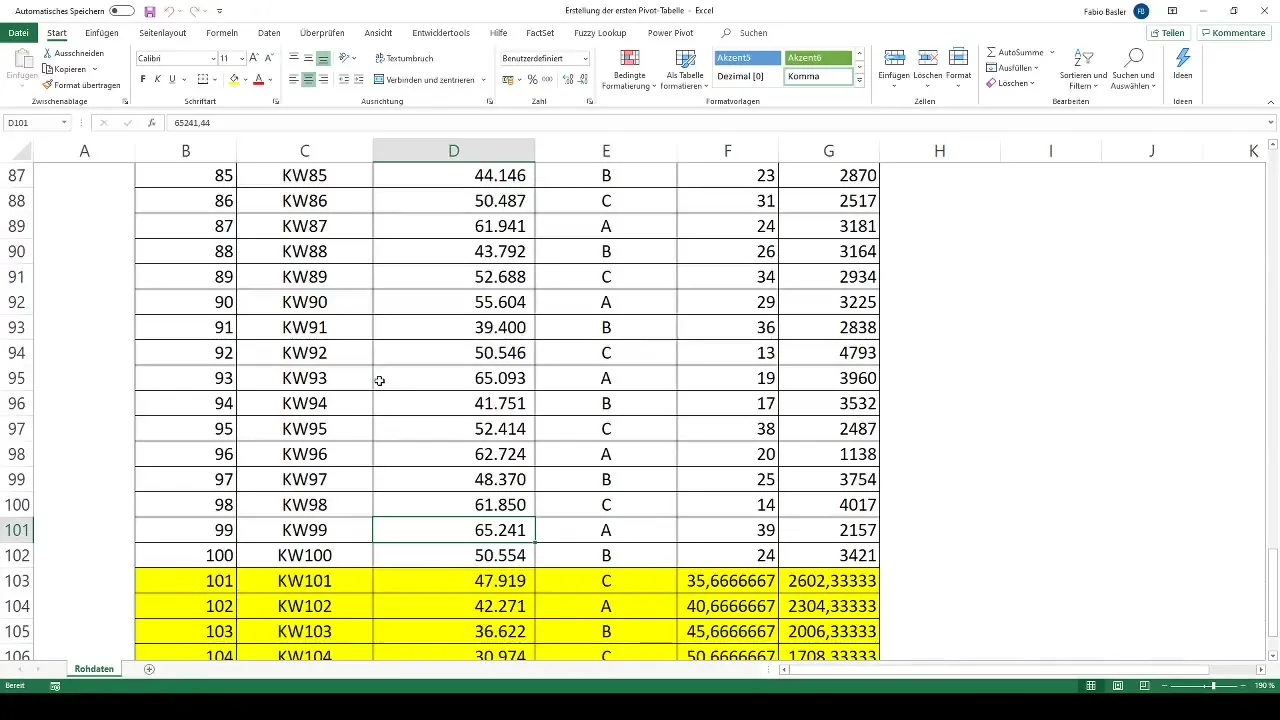
A particularly useful trick when working with pivot tables is using dynamic data sources. For instance, if you add new data not considered in the original pivot table, click on the pivot table, go to "PivotTable Tools," and select "Change Data Source." This ensures that all relevant data sources for your analysis are updated.

Step 8: Formatting Data as Table

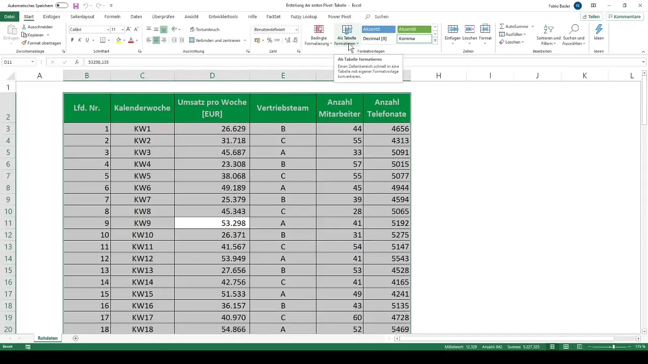
A very useful method to enhance your work with pivot tables is to format your raw data as an Excel table. This makes handling the data easier and more flexible.

Press "Ctrl + T" and make sure the first row contains the headers. This structure will make it easier for you to create pivot tables later, as Excel will automatically recognize the table as a dynamic data range.

Step 9: Create a New Pivot Table

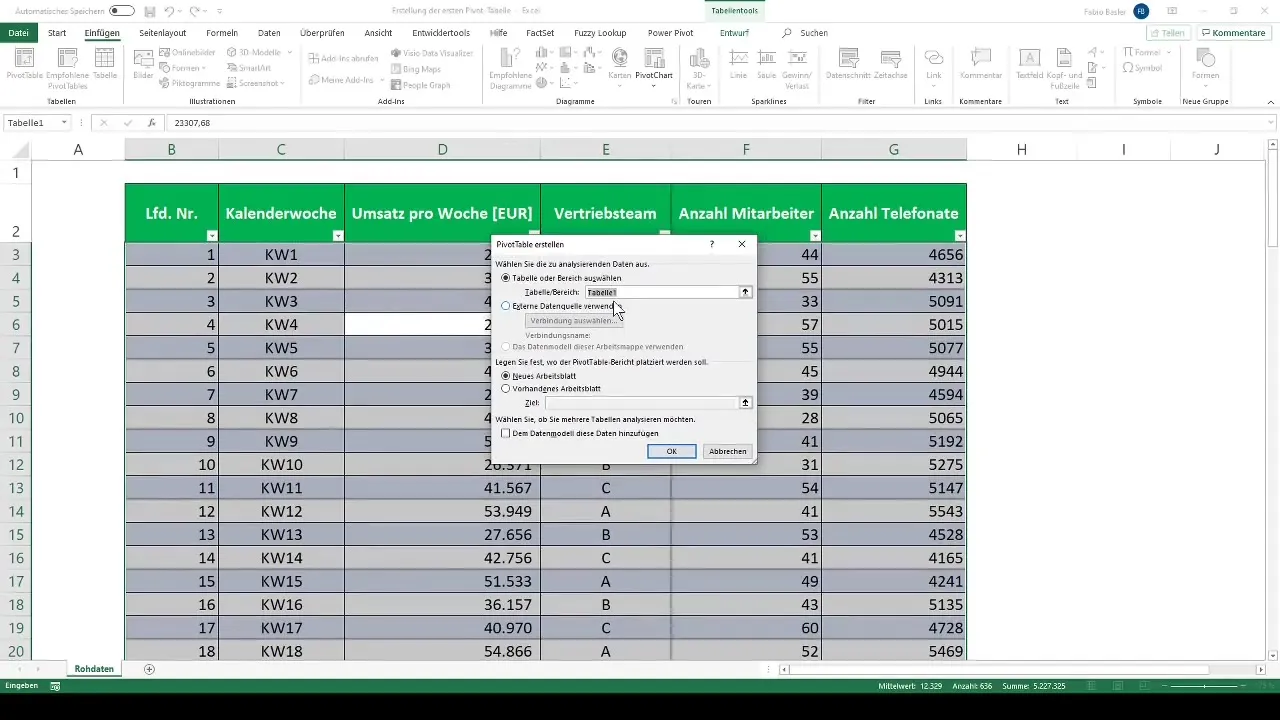
With formatted data as a table, you can now easily create additional pivot tables without having to manually select the data. Simply click on the formatted table and go back to "Insert" - "Pivot Table". Excel will adjust the data highly automatically, and the format will be much clearer.

Step 10: Automatic Update

By using a table, you are able to automatically reflect all changes in your raw data in the pivot table. Even if you add new rows, the pivot table will detect and incorporate the updates.

This significantly reduces the effort for future data analysis.

Summary

In this tutorial, you have learned the basics of creating a pivot table in Excel. Using structured data and dynamic data sources will allow you to perform more efficient analyses and manage your data dynamically. Use the tips and tricks to further optimize the process.