Create dynamic charts in Excel

There is hardly anything more exciting for a controller than presenting their data in an illustrative way. In this tutorial, I will show you how to create dynamic charts in Excel. You will learn how to use formulas from the Name Manager to make your charts interactive and individually usable. The project you will encounter in this guide consists of several steps that are essential for effective use of Excel.

Main Insights

• You will learn how to create a dynamic dropdown for months.
• The formula "OFFSET" will be explained and applied.
• The Name Manager is used to create dynamic references.
• You will create an interactive chart for different scenarios.

Step-by-Step Guide

Step 1: Create a Dynamic Dropdown for Months

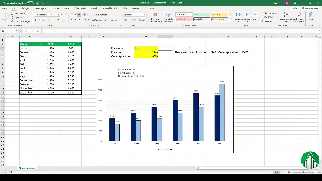
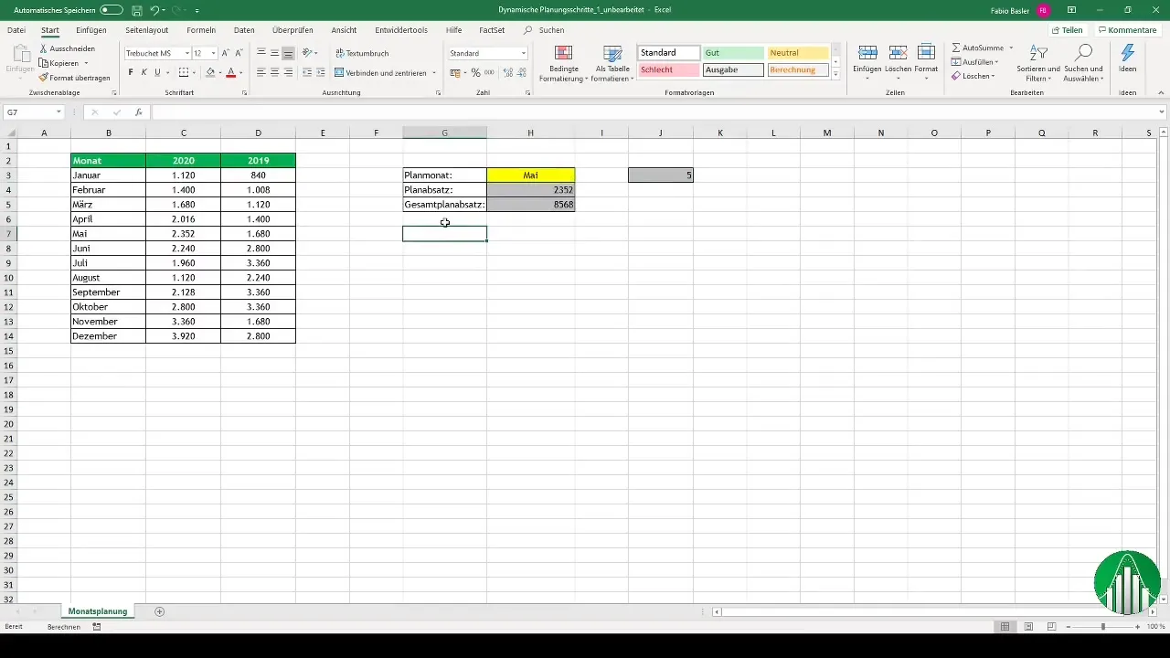
To start with our dynamic chart, you need to create a dropdown menu for the months. Go to the "Data" tab in the ribbon and select the "Data Validation" option. In the pop-up window, choose the validation criterion "List". Here, enter the month names as the source to generate a dropdown menu.

Step 2: Show Monthly Number Selection

Allow yourself to determine the month number by applying the "MATCH" formula. This uses the search criterion for the selected month within the search array to find the correct position. This way, you can display the corresponding number of the month, such as January = 1, directly.

Step 3: Retrieve Planned Sales

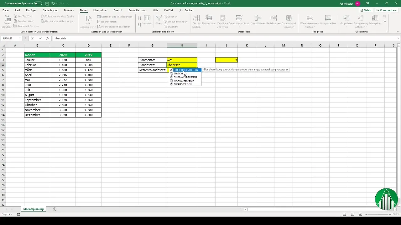
Now we want to retrieve the corresponding planned sales. Here, we use the "VLOOKUP" formula or an alternative like "INDEX" and "MATCH". In my example, you will quickly notice that the "OFFSET" formula is most effective for determining these values. It returns a reference that is offset.

Step 4: Cumulative Calculation

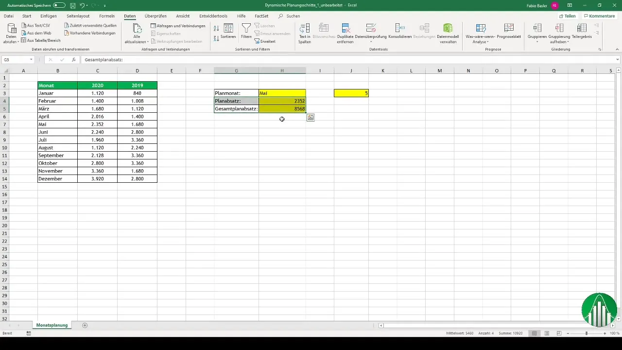
To calculate the cumulative values, we use the "SUM" formula. This way, you add up the values for the months from January to the selected month: The formula is complemented by the "OFFSET" function, so the range is dynamically adjusted. This gives you the cumulative planned sales.

Step 5: Utilize Name Manager

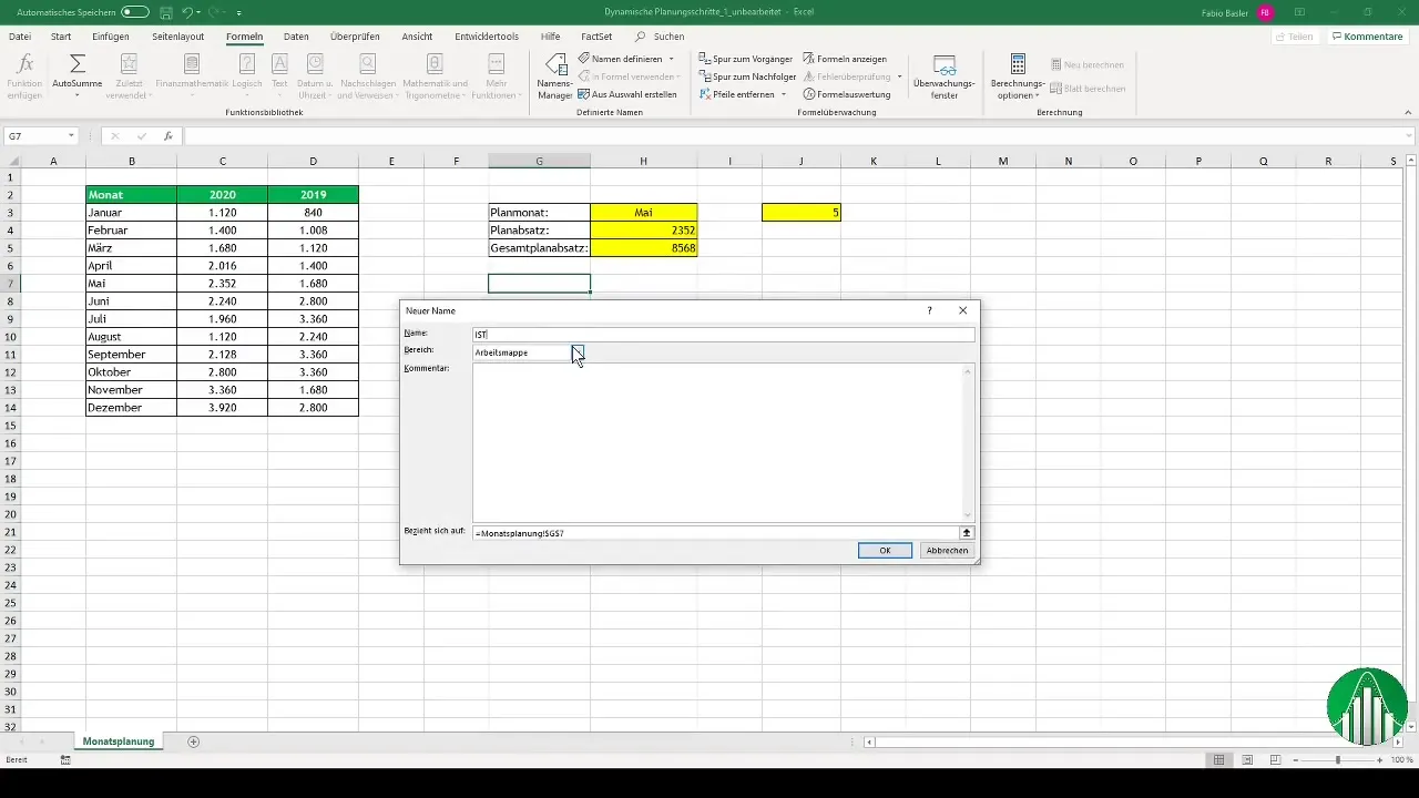
Now onto the next important aspect: the Name Manager. Through the Name Manager, you can create and manage dynamic formulas. Start by deleting all existing entries to make room for new ones. Then, create a new formula for the year 2020 and one for the previous year, 2019, and name them accordingly.

Step 6: Create Additional Formulas

Create the "OFFSET" formulas for the months, similar to the previous steps. Make sure to specify the correct parameters, so the months from 1 to 12 are accurately represented. Here, you should ensure that all formulas are well structured and named.

Step 7: Create a Chart

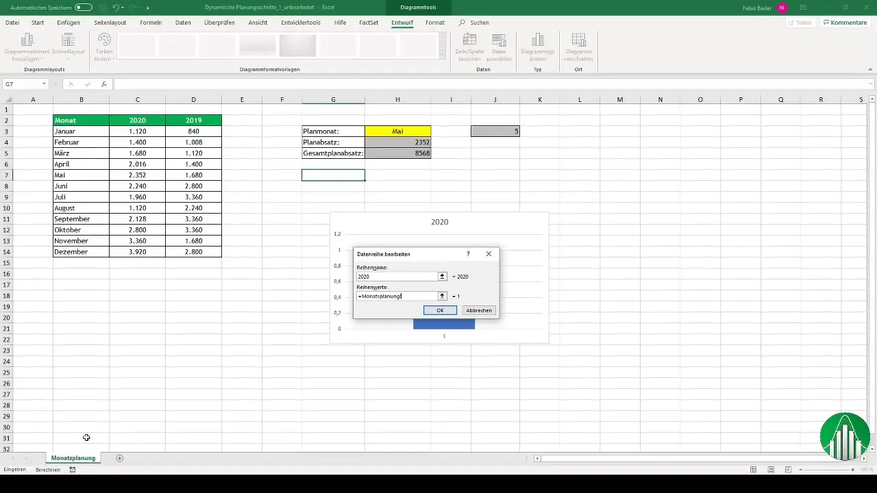
Now you can create your chart. Choose a 2D column chart to visually represent the information. Go to "Select Data" and add the series for the year 2020. It is important to precisely link the formulas to your chart, so the dynamic names from the Name Manager are correctly processed.

Step 8: Finalize the Chart

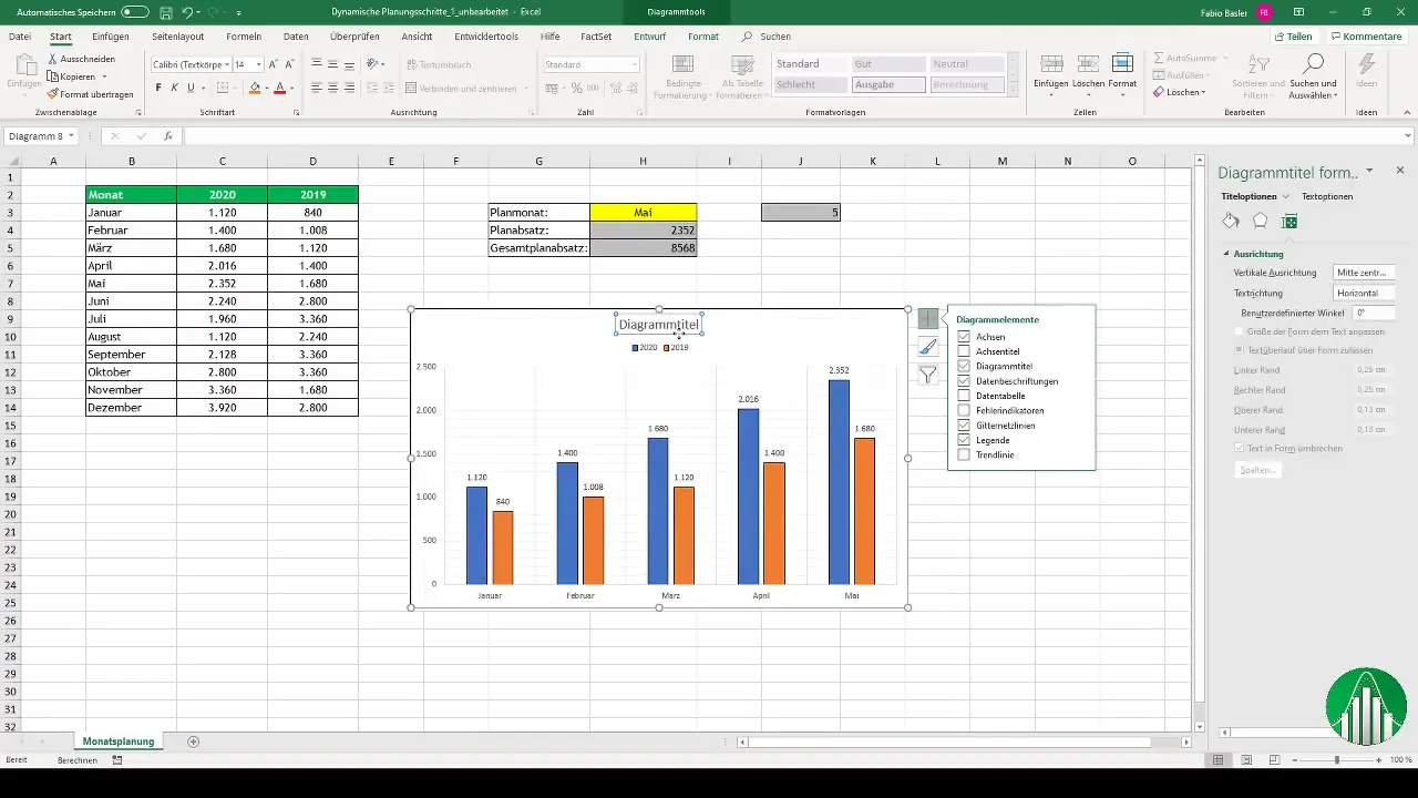
To complete the chart, add data labels and adjustments like legends and titles. You want the chart to be not only informative but also visually appealing. Creativity is key here – adapt lines and colors to optimize the chart.

Summary

In this tutorial, you were able to learn comprehensively how to create dynamic charts in Excel. You created a dropdown menu for months, retrieved the corresponding values using formulas, and generated an interactive chart. By using the Name Manager, you can have even more dynamic references, significantly improving your data presentation.