Working with functions in Excel can initially seem overwhelming, especially when it comes to filtering or searching for data selectively. One of the most common and useful functions in Excel is VLOOKUP. This function allows you to extract specific information from large datasets without having to manually search. In this guide, I will show you how to effectively use VLOOKUP, for example to filter out invoice numbers from an extensive list and display relevant information.
Key Insights
- VLOOKUP allows you to search and return specific values from a list.
- To use VLOOKUP, you need a search criterion and a matrix from which the data should be retrieved.
- The function offers the possibility to find both exact and approximate matches.
Step-by-Step Guide
1. Understanding the Basics of VLOOKUP Function
First, you need to understand what VLOOKUP actually does. This function scans the first column of a specified matrix and looks for a specific value, then returns a value from another column in the same row.
2. Create Sample Data
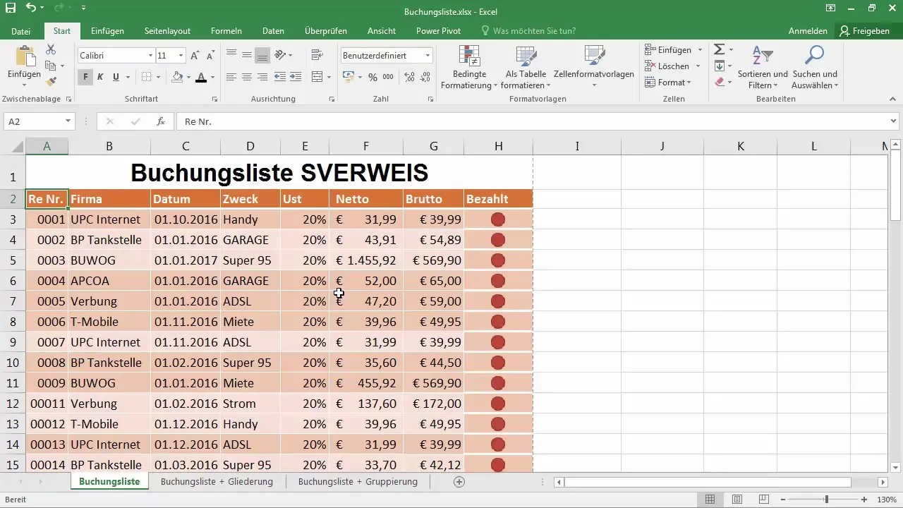
Open an Excel workbook and create a sample table with invoice numbers, company names, invoice dates, net amounts, and purposes. Make sure this table is structured so that VLOOKUP works correctly.
3. Set Search Criterion
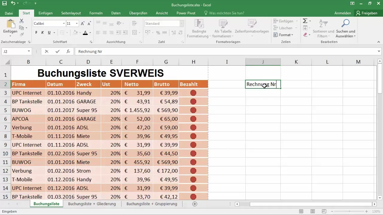
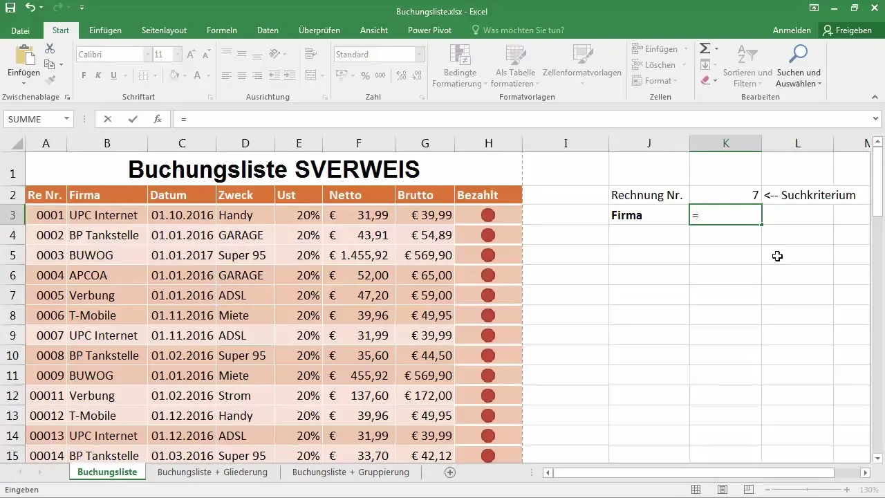
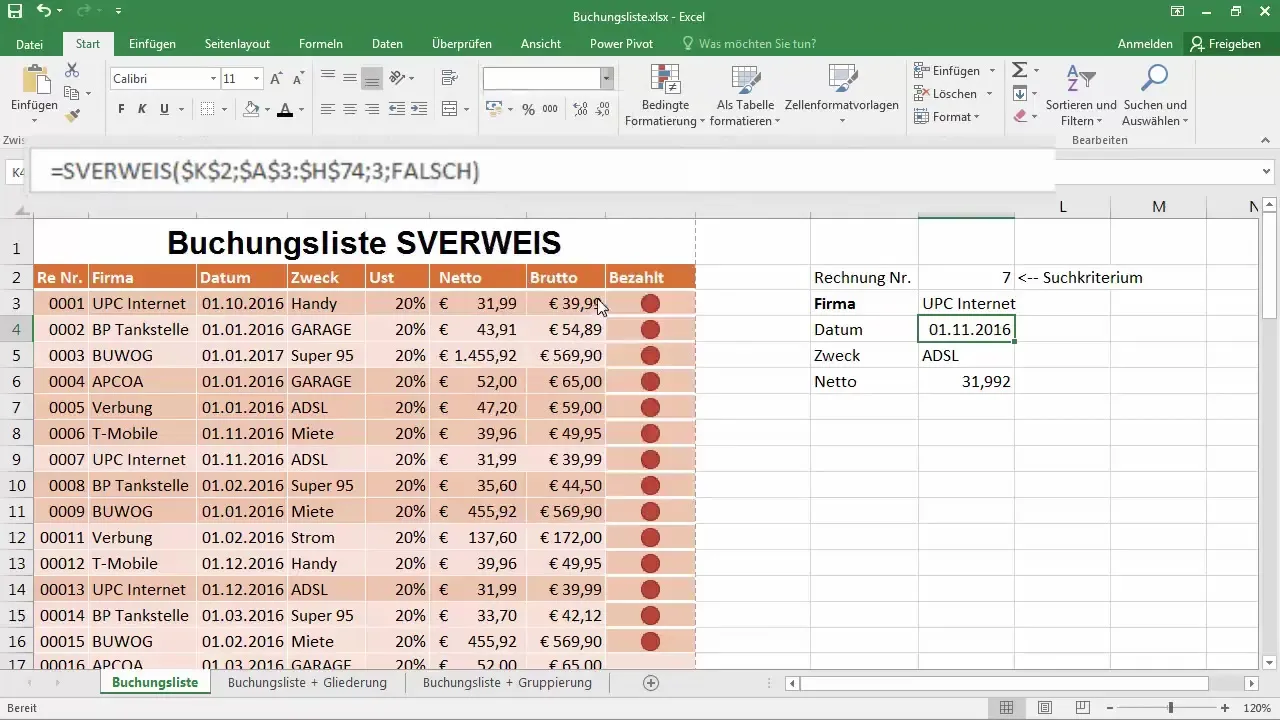
Select the field where you want to enter the invoice number. For example, you can directly enter the invoice number "007" into the cell that serves as the search criterion.
4. Enter VLOOKUP Function
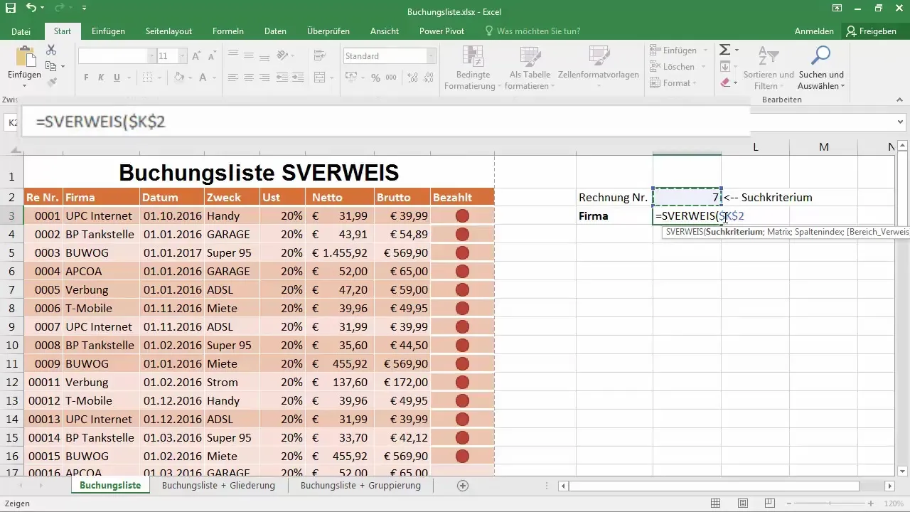
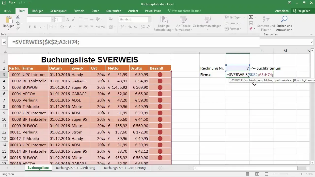
Go to the cell where the corresponding company name should be displayed, and start entering with "=VLOOKUP(". Here, you specify your search criterion, which relates to the invoice number, and the matrix you want to search through.
5. Set the Reference
Now you need to set the reference to your search criterion. It is important to set the cell with the invoice number as an absolute reference so that this value is not changed when copied. You can do this by pressing the "F4" key.
6. Select Matrix
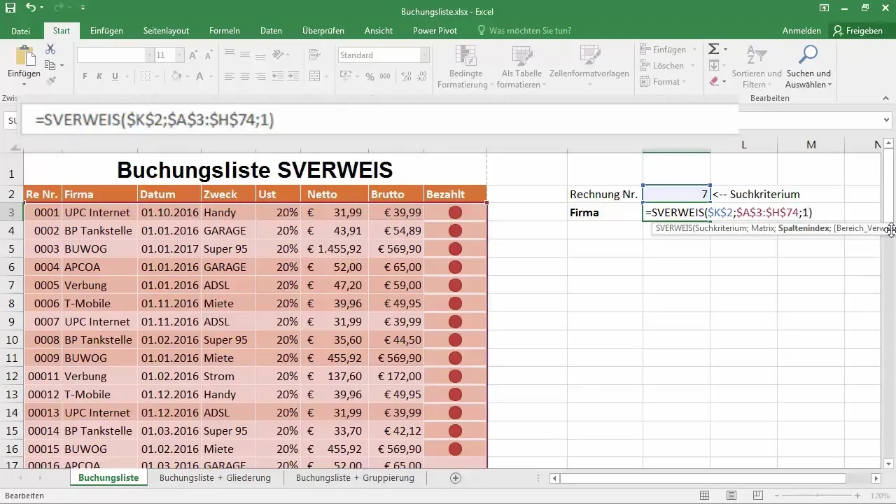
Then, select the matrix in which Excel should search for the invoice number. The matrix should include all relevant columns from which you want to retrieve data.
7. Specify Column Index
After selecting the matrix, specify the column index. For example, if the invoice number is in the first column and you want to return the company name from the second column, enter the value "2."
8. Define Match
Now, you need to decide whether you want an approximate or exact match. For an exact search, enter "0." This will only output an exact finding of the invoice number.
9. Complete the Function
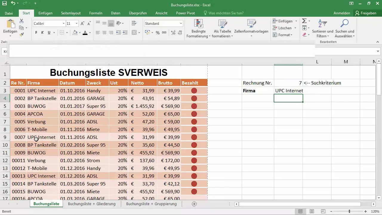
Confirm the entry with "Enter." After entering the VLOOKUP, you should now see the corresponding company name associated with the invoice number "007."
10. Use AutoFill Feature
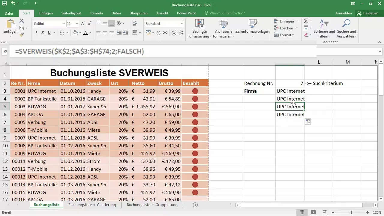
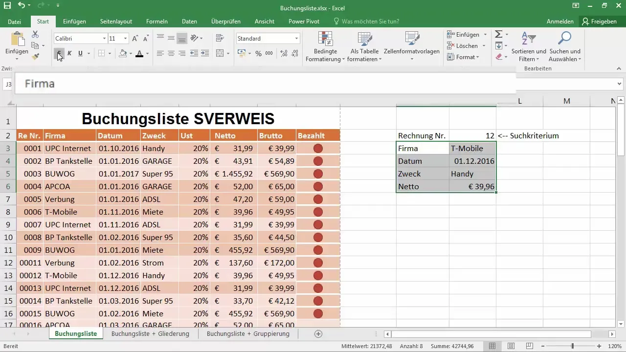
You can use the AutoFill function to apply VLOOKUP for other invoice numbers in the same field. Make sure to adjust the column index for the desired data (e.g., invoice date, net amount) accordingly.
11. Adjusting Data Formats
If the displayed data does not appear in the desired format (e.g. date and currency values should be displayed correctly), change the cell formatting accordingly by selecting the correct format.
12. Testing with Different Invoice Numbers
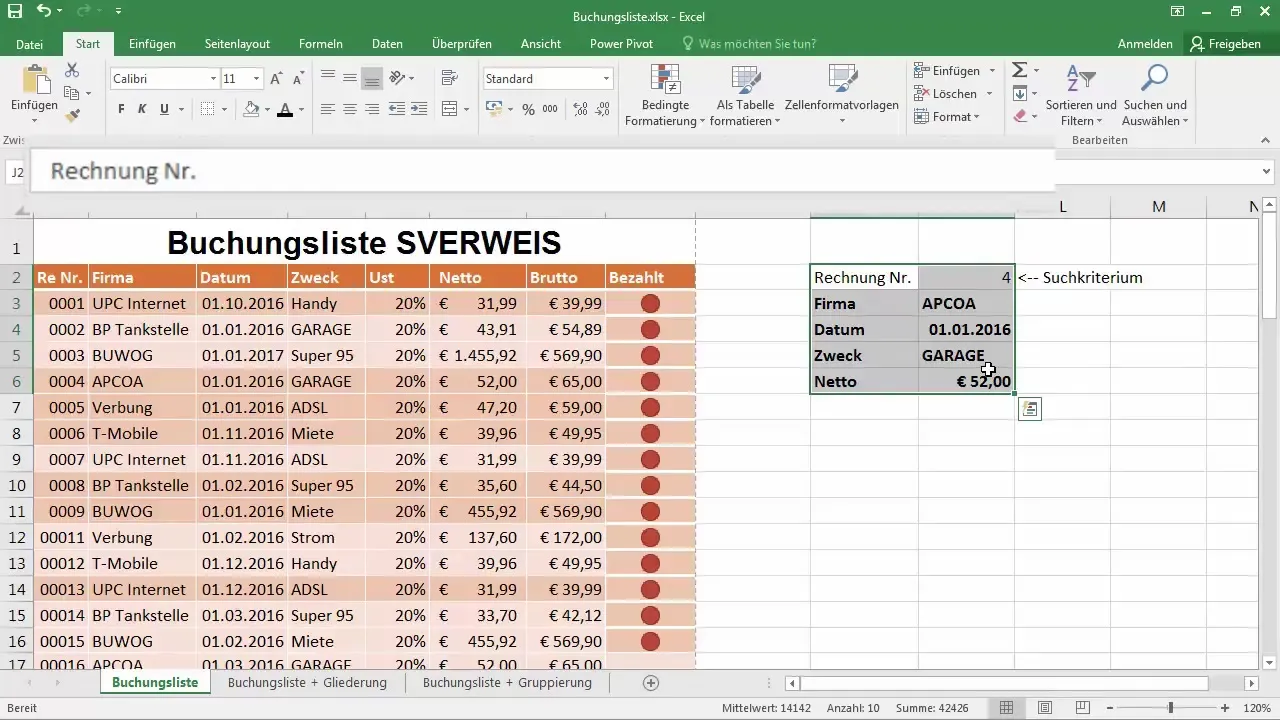
Test the function by entering other invoice numbers in the search field. You will see that the other data is automatically updated.
13. Application of VLOOKUP in Practice
Remember that you can use VLOOKUP to create a user-friendly search mask in your Excel document. This allows you or users to quickly find and display relevant data without having to scroll through large amounts of data.
14. Next Steps
In the next chapter, you can learn how VLOOKUP can be used in combination with comparison operators to perform dynamic searches. This can expand the application of the function and make it easier to adapt to different data sets.
Summary
VLOOKUP is a powerful tool in Excel to selectively extract data from extensive tables. By structuring your data clearly and correctly applying the VLOOKUP function, you can simplify the overview of important information. Experiment with the various settings of the VLOOKUP function to fully leverage its capabilities.
Frequently Asked Questions
How does the VLOOKUP function work in Excel?The VLOOKUP function searches a table for a search criterion in the first column and returns a value from a specific column in the same row.
Can VLOOKUP be used in other worksheets?Yes, you can set up VLOOKUP to retrieve data from other worksheets as long as you correctly reference the table.
What happens if the invoice number is not found?If the invoice number is not found, the function returns an error value. You can address this with error handling in Excel.
Should the matrix be sorted in ascending order?For exact matching, sorting is not necessary, but for approximate matches, the first column must be sorted in ascending order.
How can I automatically apply VLOOKUP to other cells?You can use the Autofill function to automatically apply VLOOKUP to other cells by dragging the formula down.


