Mean analysis of sales numbers in Excel

Statistical indicators are essential for making informed decisions and analyzing relevant data. In this guide, you will learn how to perform the mean calculation for sales data of smartphones and notebooks in Excel. Following a clearly structured approach, you will learn how to successfully implement the necessary steps for the calculation and how to effectively interpret this information.

Main Insights

• Means can help you compare sales performance of products.
• Metric scale levels are crucial for calculating means.
• With Excel, you can use both manual mean calculations and Pivot tables to analyze data.

Step-by-Step Guide

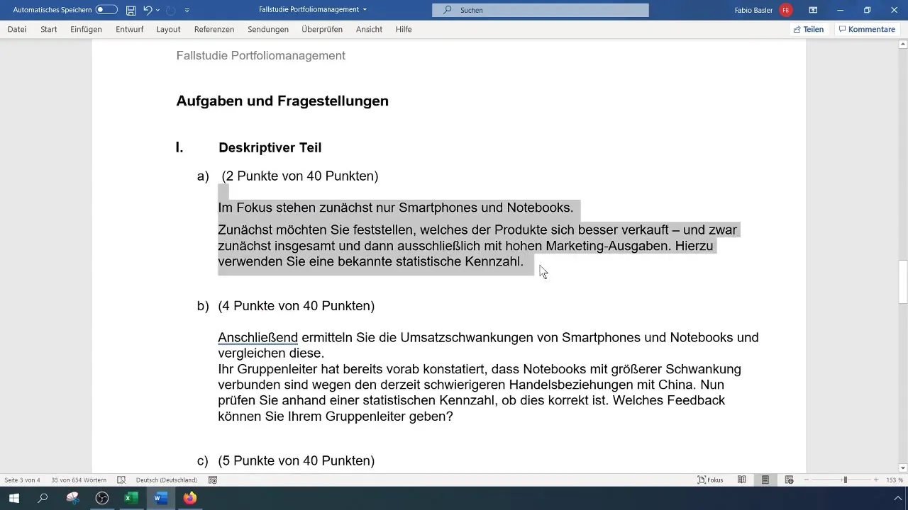
Prepare sales data

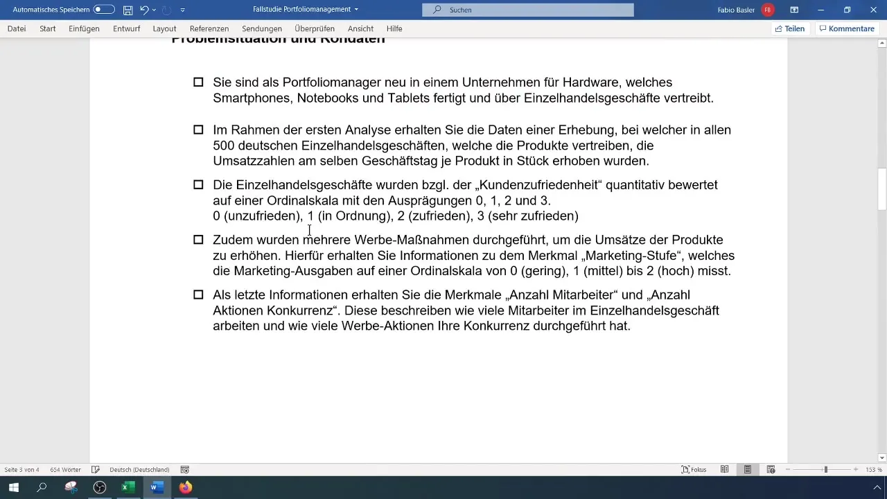
To analyze the sales figures of smartphones and notebooks, start by structuring the data you have available. Ensure that the sales figures are accurately captured and ready on an Excel worksheet.

Copy and paste data

Select the relevant sales data for smartphones and notebooks. You can do this by right-clicking and "Copy" or by pressing the Ctrl + C key combination. Then paste the data into Worksheet A to have a clear workspace.

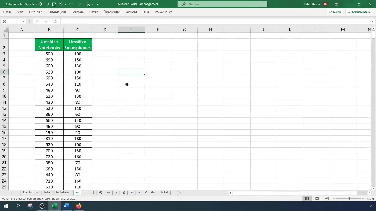
Identification of relevant statistics

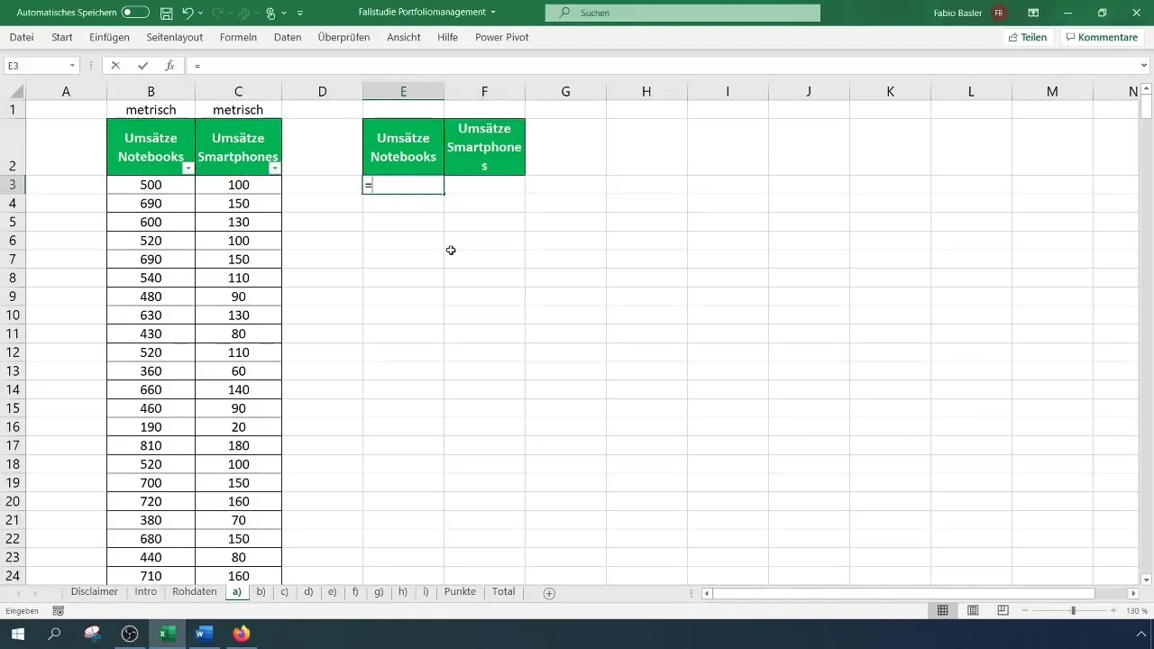
Here, the selection of statistical indicators comes into play. The mean indicator is particularly suitable as it helps you compare the sales of products. Consult your formula collection to ensure you are using the correct mean indicators.

Calculation of the arithmetic mean

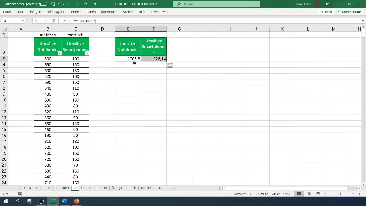
Now the exciting part begins, calculating the arithmetic mean. Use the Excel formula =AVERAGE() and select the range of sales figures for notebooks. These data will now be processed to show you the average sales.

Faster data selection

To speed up data selection, you can use a key combination: Hold down the Shift key and select the desired range. This makes data entry more efficient and allows you to capture sales figures more quickly.

Calculation for smartphones

Repeat the previous step for smartphones to determine their average sales. Now you will know which product sold better overall.

Filtering by high marketing expenses

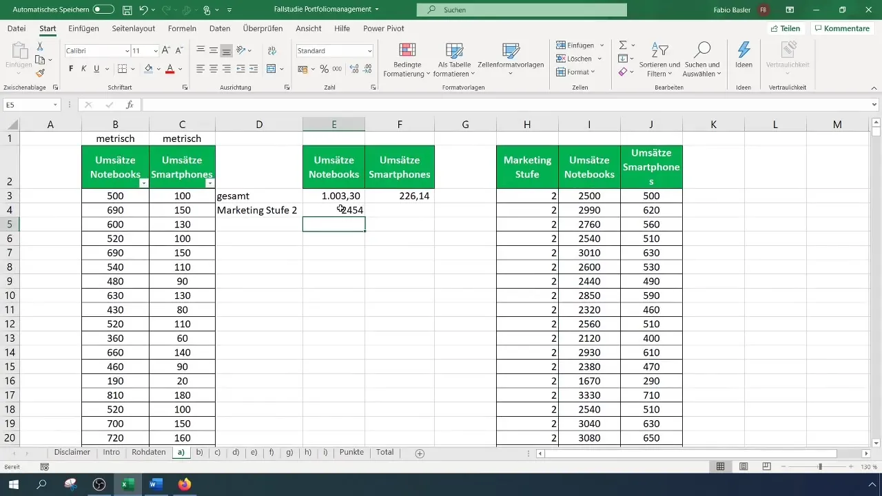
For more detailed analysis, marketing expenses are now taken into account. Filter the sales data by Marketing Level 2 to see how high marketing expenses affect sales.

Calculation of the mean for filtered values

The next steps involve calculating the mean for the filtered data. Once again, use the =AVERAGE() formula, but this time only for the filtered sales of notebooks and smartphones with high marketing expenses.

Pivot table for analysis

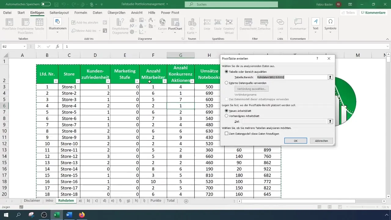
To analyze the data more efficiently, you can create a Pivot Table. Go to "Insert" in the menu bar and select "PivotTable". This allows you to compare values for notebooks and smartphones.

Adjustment of the Pivot Table

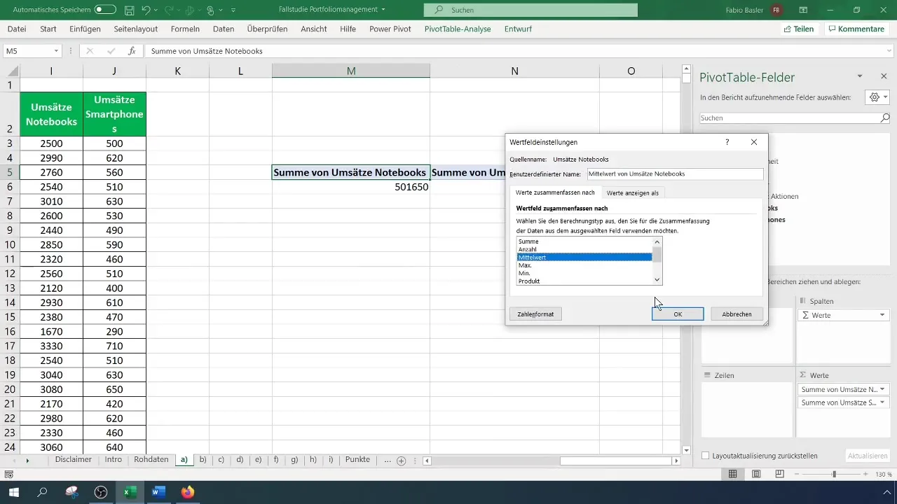
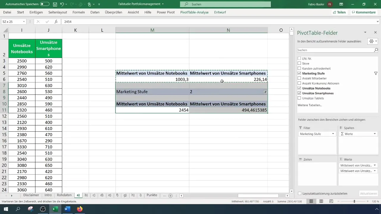
Change the sum setting in the value fields of the Pivot Table to "Mean". This will give you a consolidated overview of the mean values of the products based on the sales figures.

Processing the Pivot Table Data

Copy the pivot table and paste it below the original table. Then you can add another filter to display the results only for Marketing Level 2.

Summary

The step-by-step guide to mean analysis in Excel presented here ensures that you effectively analyze sales of smartphones and notebooks. By using the techniques provided to calculate the mean, you establish a solid foundation to optimize your sales strategies.