Correlation analysis and Pearson coefficient in Excel

The analysis of relationships is a fundamental skill that is indispensable in many scientific and business fields. Using Excel, you can determine the Pearson correlation coefficient to measure relationships between variables quantitatively. In this guide, I will show you step by step how to perform a correlation analysis for the sales behavior of smartphones and notebooks in Excel. This process not only demonstrates the application of statistical concepts but also the easy handling of Excel for data analysis.

Key Takeaways

• The Pearson correlation coefficient provides a quantitative assessment of the relationship between two variables.
• Know the different methods for calculating the correlation coefficient in Excel.
• Visualizing the results through charts facilitates understanding the relationships between variables.

Step-by-Step Guide

The following steps show you how to calculate the Pearson correlation coefficient in Excel. We focus on the sales of smartphones and notebooks to demonstrate a clear and practical application.

To start the correlation analysis, first open a new Excel workbook or use an existing one where the relevant data is present.

First, make sure that the respective sales figures of smartphones and notebooks are entered in two separate columns. These columns form the data basis on which the analysis is built. Ensure that the data is entered completely and correctly to avoid distorted results.

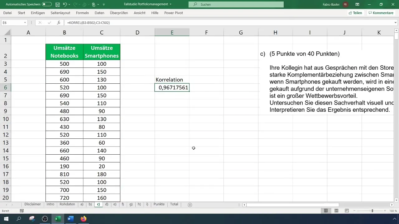
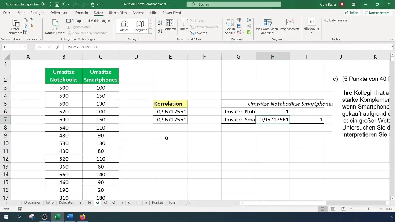
After entering the data, select the two columns with the sales figures. To calculate the correlation coefficient, enter the formula =CORREL() in an empty cell, followed by the two data ranges. This function will calculate the Pearson correlation coefficient based on the selected data.

When you use the formula =CORREL(Range1, Range2), select the entire range of the column representing notebook sales, followed by the range of smartphone sales. The output will give you the correlation value between these variables. A high correlation, such as 0.96, indicates a strong positive relationship.

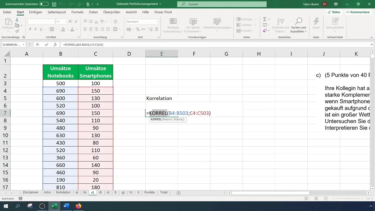
In addition to the CORREL function, you can also use the =PEARSON() function, which provides an identical result. Enter this function in a similar manner as before and select the data ranges to determine the correlation.

Another interesting way to perform correlation analysis is through the data analysis function in Excel. To activate this function, go to the "File" menu and then to "Options". Under the Add-Ins section, you can enable the Data Analysis option if it is not already activated.

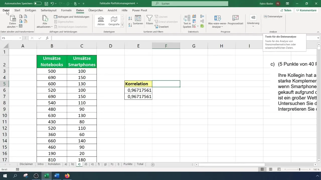
After activating the Data Analysis function, choose "Data Analysis" from the ribbon and click on "Correlation". An input form will open where you define the input range for the data, including the column headings.

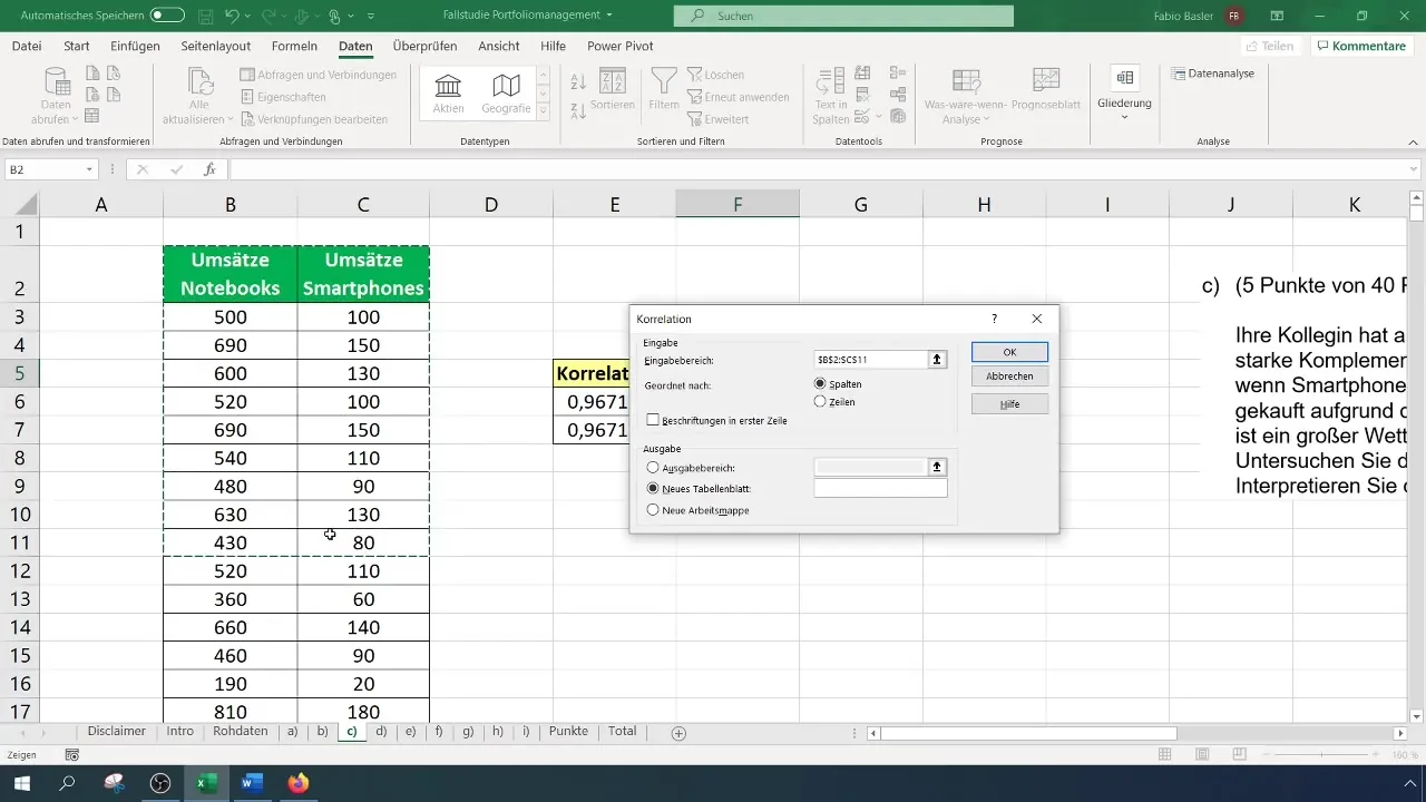
When defining the output range, select an empty cell where the results will be displayed. By confirming the input, a correlation matrix will be generated showing all relationships within the specified data. Here, you will again notice the high correlation of about 0.96.

To visually represent the relationship between variables, a scatter plot is suitable. Select an empty cell and insert an XY chart. Right-click on the chart and select "Select Data".

Add the sales figures for both smartphones and notebooks. This visual representation will show you how the points are distributed between the two variables and illustrate the relationship through clustering effects.

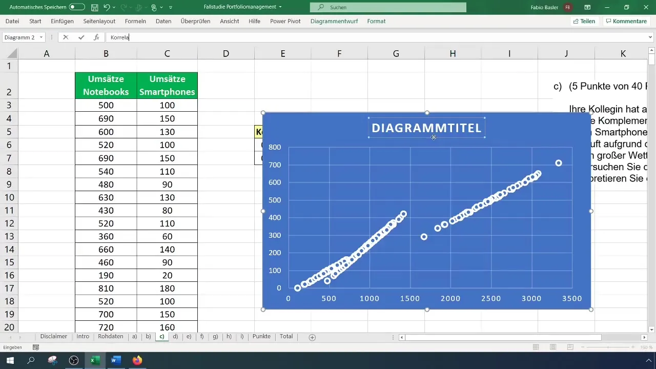
An additional way to analyze the relationship is to add a trendline to the chart. Click on the plus sign in the top right of the chart and enable the trendline option. You can also display the formula and coefficient of determination R² for further analysis.

The coefficient of determination indicates how well the trend line describes the data and is the square value of the correlation coefficient. An R² of about 0.935 reinforces the strength of the relationship between notebooks and smartphones, supporting the correlation previously calculated.

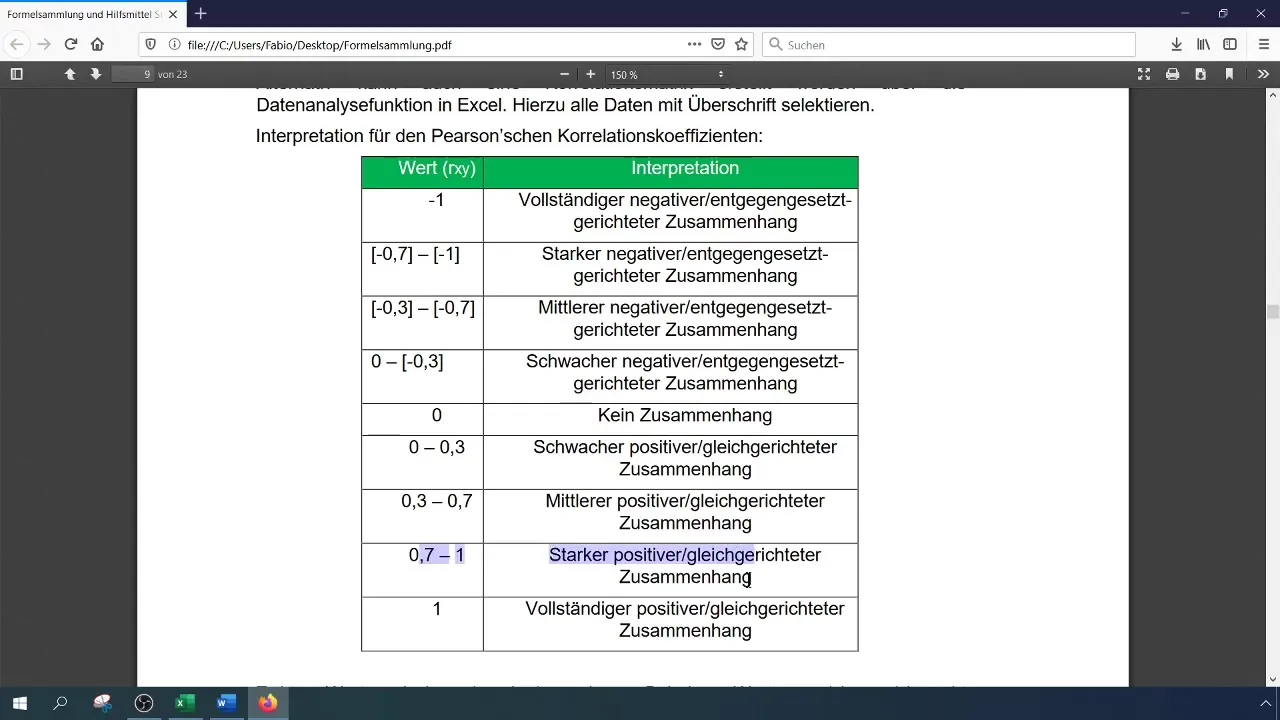
Finally, it is important to interpret the results. Values above 0.90 indicate a strong positive correlation, meaning that an increase in one revenue area corresponds to an increase in the other. In this case, the relationship between smartphone and notebook revenues is extremely strong.

Summary

In this guide, you have learned how to calculate and interpret the Pearson correlation coefficient in Excel. Through the different methods, multiple ways have been shown to quantitatively and visually represent the correlation between variables. This gives you the opportunity to analyze real data and gain important business insights.