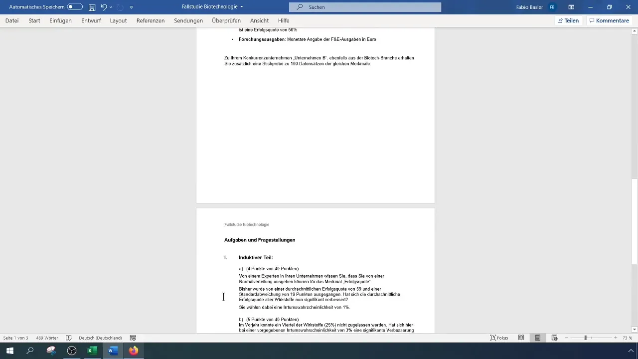
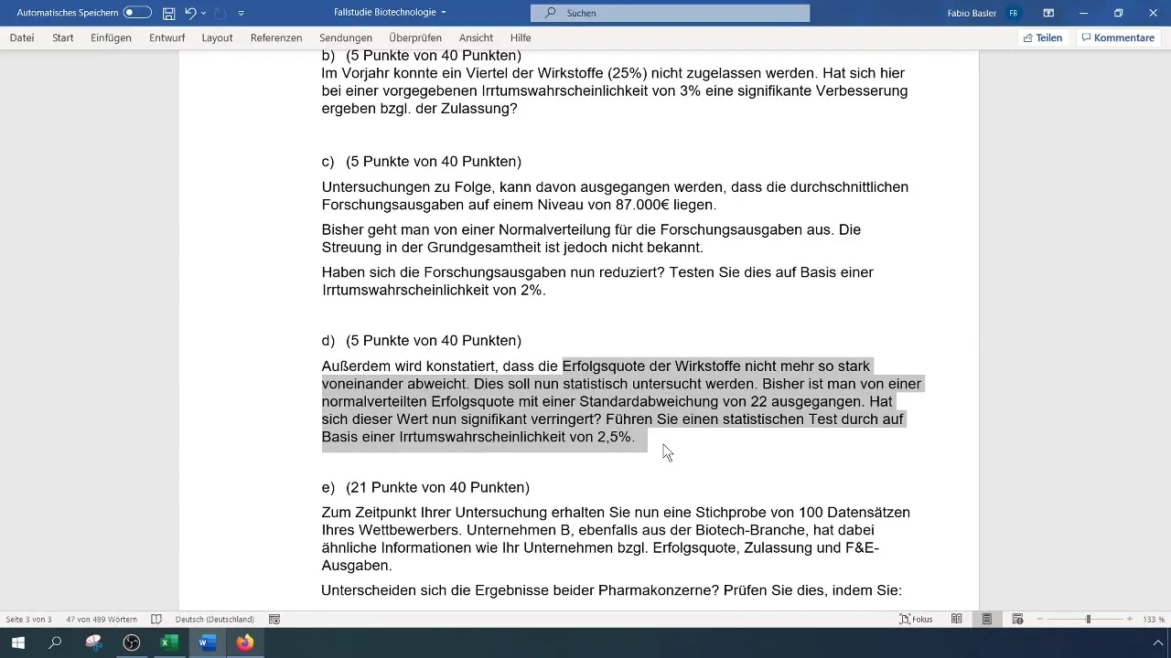
As part of statistical analyses, hypothesis testing is a central tool that allows you to examine various assumptions about a dataset. In this guide, you will learn how to conduct a single-sample test for variance in Excel. You will learn both the theoretical foundations and the practical steps to test for significant changes in the variance of your sample.
Key Takeaways
- The test examines whether a known standard deviation significantly deviates from a new one.
- The hypothesis test for variance is carried out using a single-sample approach.
- The calculation involves setting hypotheses, determining the test statistic, and comparing it with a critical value from the chi-square distribution.
Step-by-Step Guide
Step 1: Preparing the Dataset
First, you need to import your dataset into Excel or enter it manually. The dataset should contain the values relevant for calculating the variance. To do this, open Excel and create a new table. Enter the values into a column.

Step 2: Calculating the Standard Deviation and Variance
To calculate the variance, you need to use the standard deviation of your sample. If you have a known standard deviation (in this case 22), square this value to obtain the historical variance (σ0²). Use the following formula:
Variance (σ0²) = (Standard Deviation)²
You can easily do this in Excel by entering it into a cell.
Step 3: Formulating the Hypotheses
Now, you will formulate your null hypothesis (H0) and the alternative hypothesis (H1). The null hypothesis states that the variance is equal to the known variance, while the alternative hypothesis posits that the variance has been significantly reduced. Write this down:
- H0: σ² = 484
- H1: σ² < 484

Step 4: Calculating the Test Statistic
The test statistic (χ²) is determined by the following formula:
χ² = (n - 1) * (σ1² / σ0²)
Here, n is the number of data points and σ1 is the estimated standard deviation from your sample. To calculate this in Excel, you can reference the corresponding cells.

Step 5: Determining the Critical Value
To find the critical value for the test, you need the chi-square distribution. You can calculate this value in Excel using the CHISQ.INV() function, where you use the desired significance level (here 2.5% for a one-tailed test) and the degrees of freedom (n-1).
Step 6: Comparing the Test Statistic with the Critical Value
Now compare the calculated test statistic (χ²) with the critical value. If the test statistic is smaller than the critical value, you can reject H0. This means that there is a significant difference and the variance has been reduced.
Step 7: Drawing Conclusions
Based on your test, you can now formulate a conclusion. If H0 is rejected, you should clarify that the variance in your population is significantly lower than the original variance. Document your results and present them in a report.
Summary
In this guide, you have learned how to effectively conduct a single-sample test for variance in Excel. By applying the theoretical foundations in practice, you will be able to gain insights into your data.
Frequently Asked Questions
How is variance calculated in Excel?Variance can be calculated in Excel by using the formula VAR.P() for the population or VAR.S() for a sample.
What is the difference between H0 and H1?H0 is the null hypothesis, which assumes no difference. H1 is the alternative hypothesis, which postulates a significant difference.
What do I do if H0 is not rejected?If H0 is not rejected, it means that the data do not provide enough evidence to claim that the variance significantly deviates from the known variance.


