Using Excel for managing business data can be incredibly beneficial, especially when it comes to financial analysis. In this guide, you will learn how to use the Subtotal function in Excel to calculate automatic subtotals for your sales list. Specifically, we will show you how to present and highlight quarterly figures clearly and in color.
Main Insights
- The Subtotal function allows for easy calculation of subtotals based on specific criteria, such as quarters.
- Grouping data can significantly improve the clarity of your analyses.
- Conditional formatting can be used to visually highlight important results.
Step-by-Step Guide
1. Open the sales list
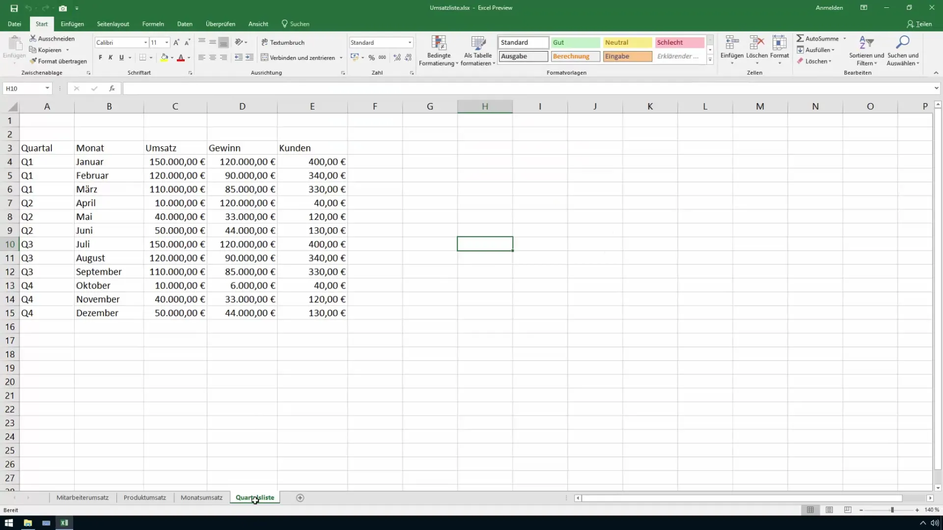
Start by opening your sales list in Excel. You will need a file that contains all relevant data, such as months, sales, profits, and customers.
2. Select the relevant data range
The quarterly list lists the months, sales, profits, and the quarters. Now select the range you want to use for calculating the subtotals, such as the values of the quarters.
3. Apply the Subtotal function
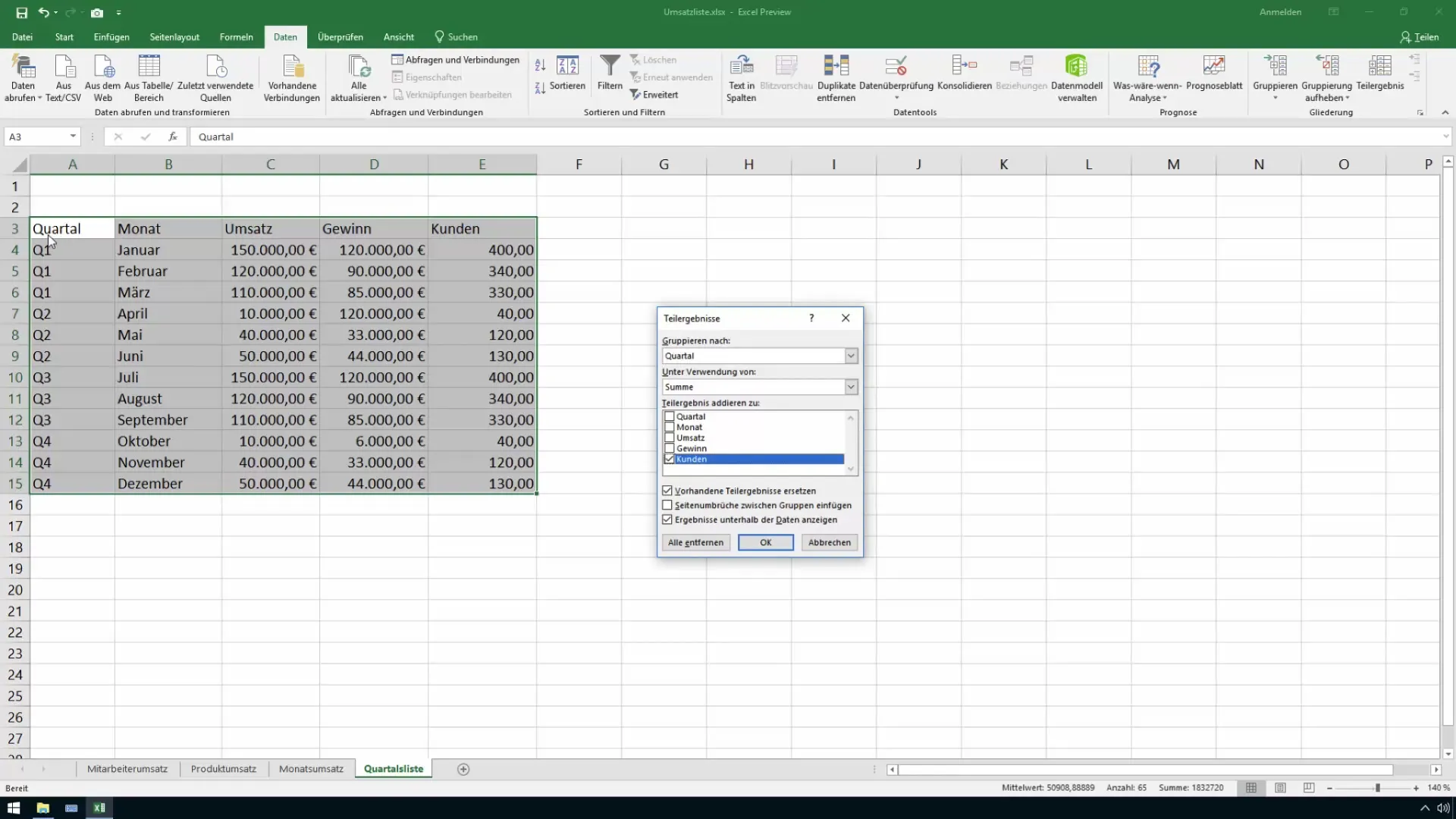
To use the Subtotal function, go to the "Data" tab in the menu bar and look for the "Outline" section. There you will find the option "Subtotal." Click on it to open the corresponding menu.
4. Group by quarter
Now you need to specify that grouping should be done by quarters. Choose "Quarter" as the grouping criterion. This means that all values belonging to the same quarter will be summarized.
5. Set the use of the Sum function
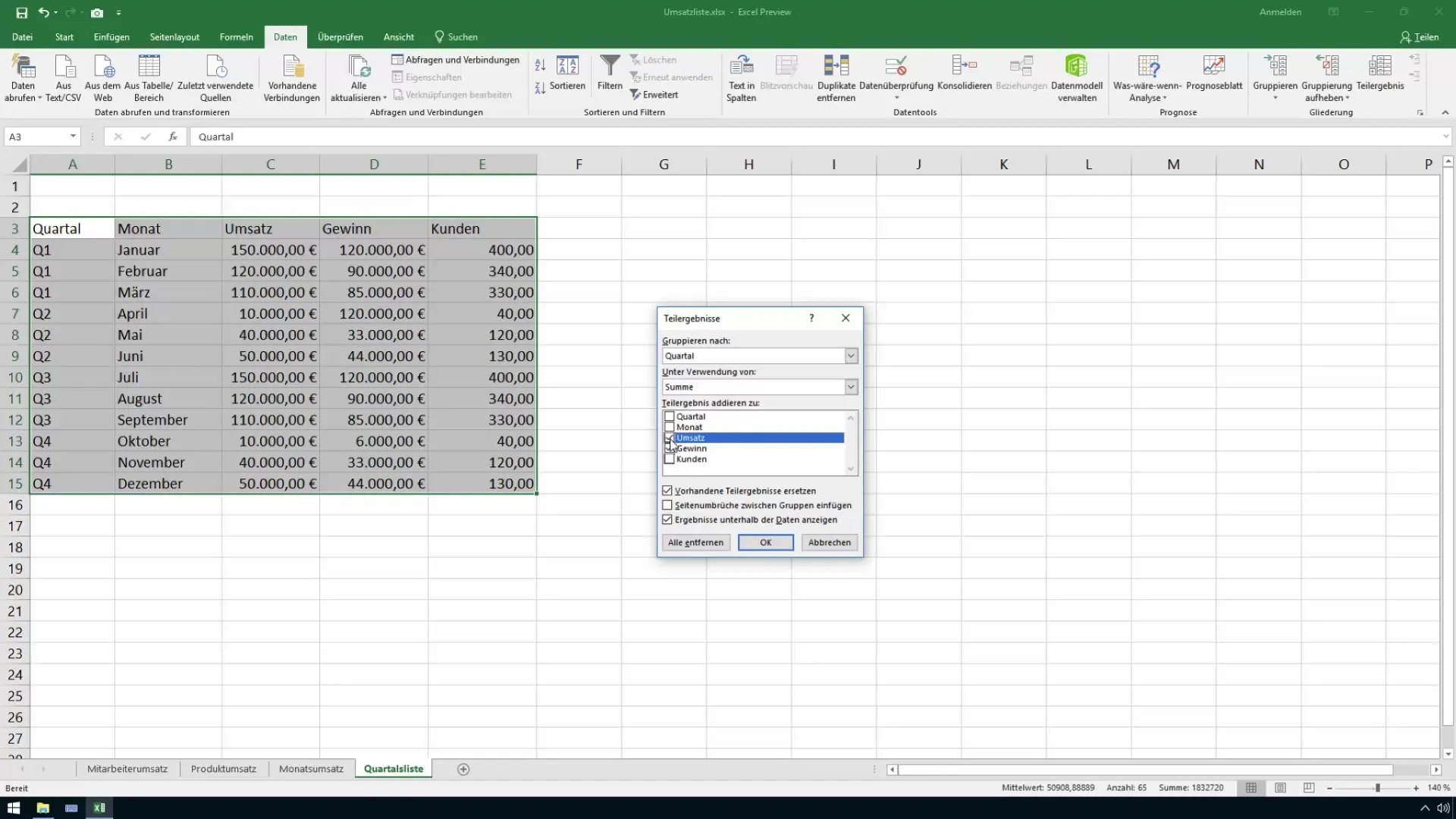
You will also be prompted to select a function for calculation. Choose "Sum" to add both profits and sales for each quarter. Confirm these entries by clicking "OK."
6. Review the results
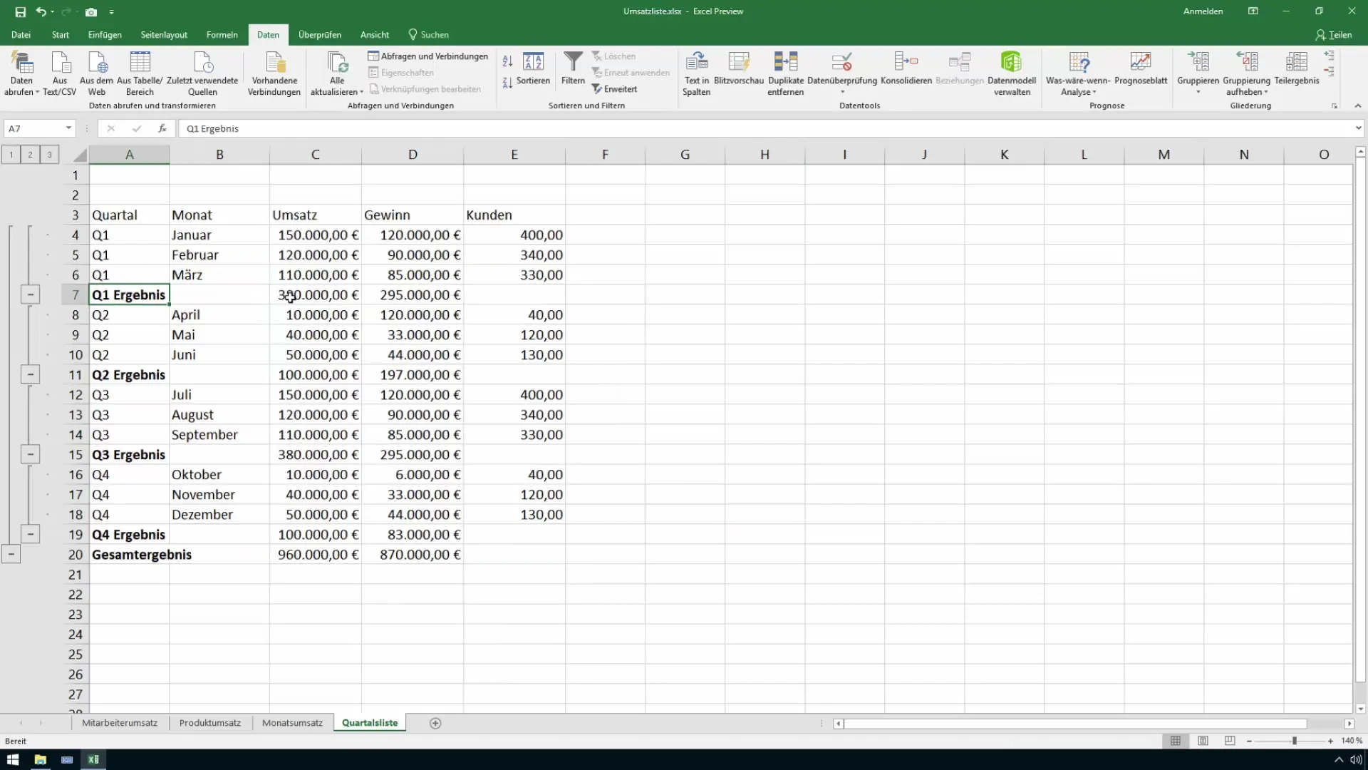
After clicking "OK," you will see the estimated subtotals for each quarter, including the total figures for sales and profits. This way, you quickly get an overview of the financial situation.
7. Visualize the results
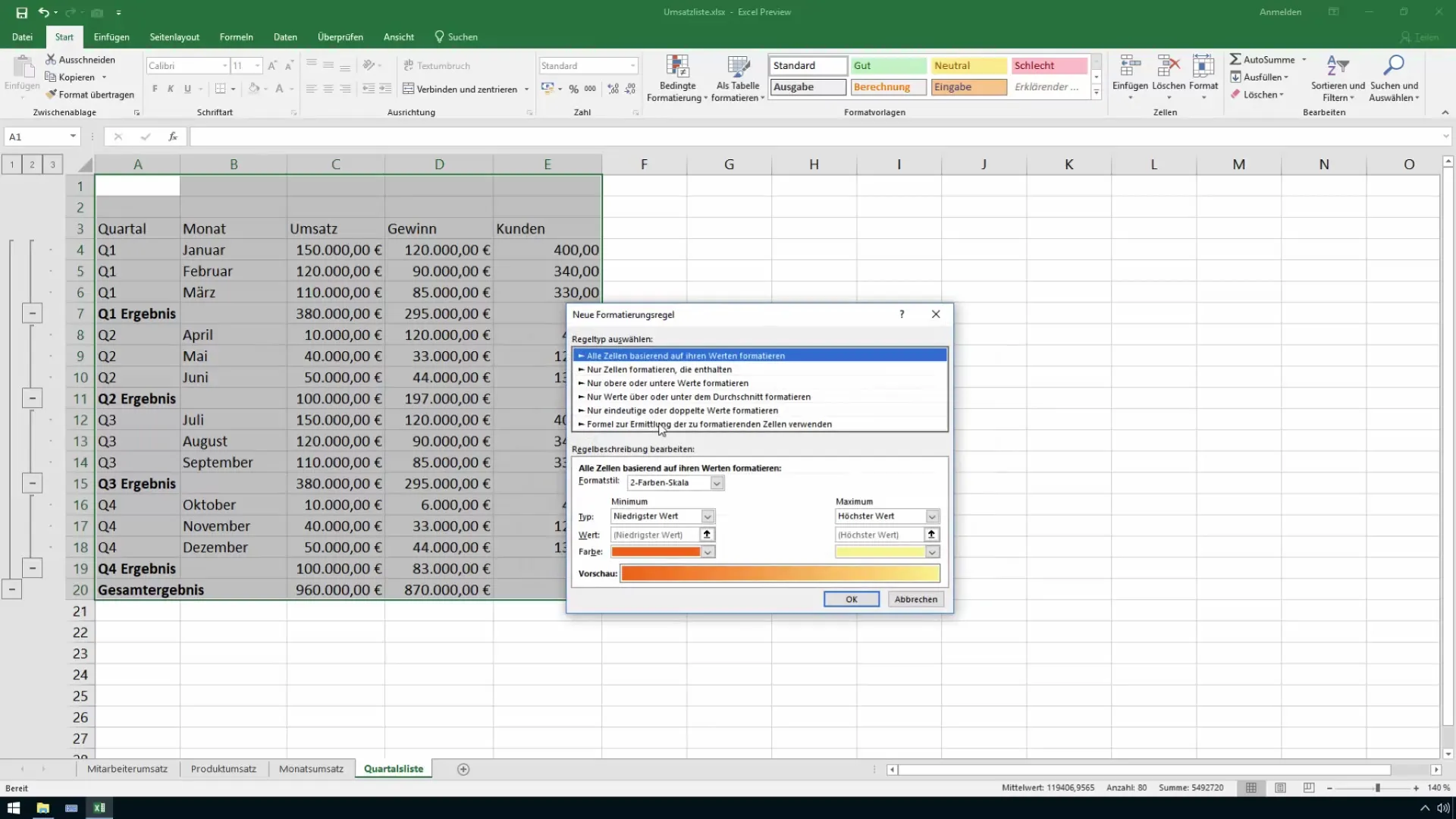
To make the quarterly results visually appealing, you have the option to highlight them in color. Select the relevant cells and go to the "Home" tab. Choose the option for "Conditional Formatting."
8. Adjust conditional formatting
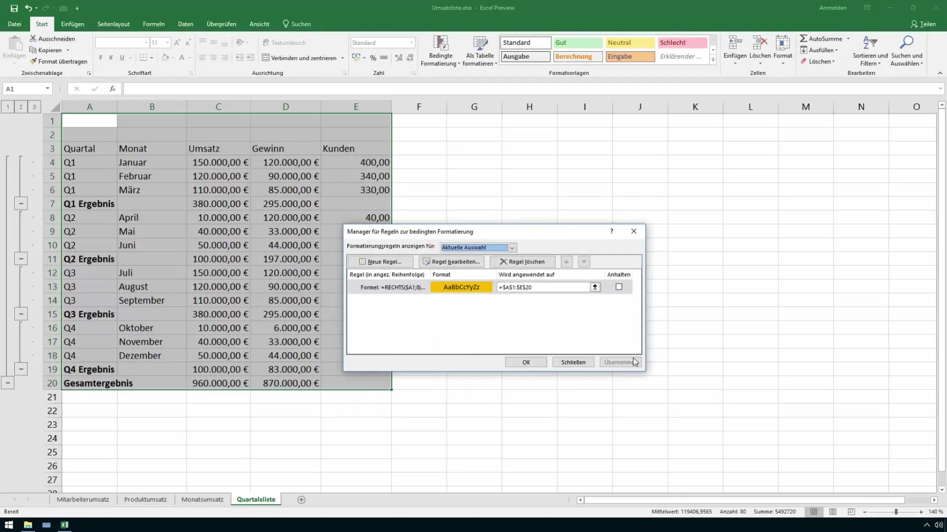
Here you have the opportunity to create a new rule for formatting. Choose the option "Use a formula to determine which cells to format." Enter the formula that highlights the results according to criteria.
9. Define formatting
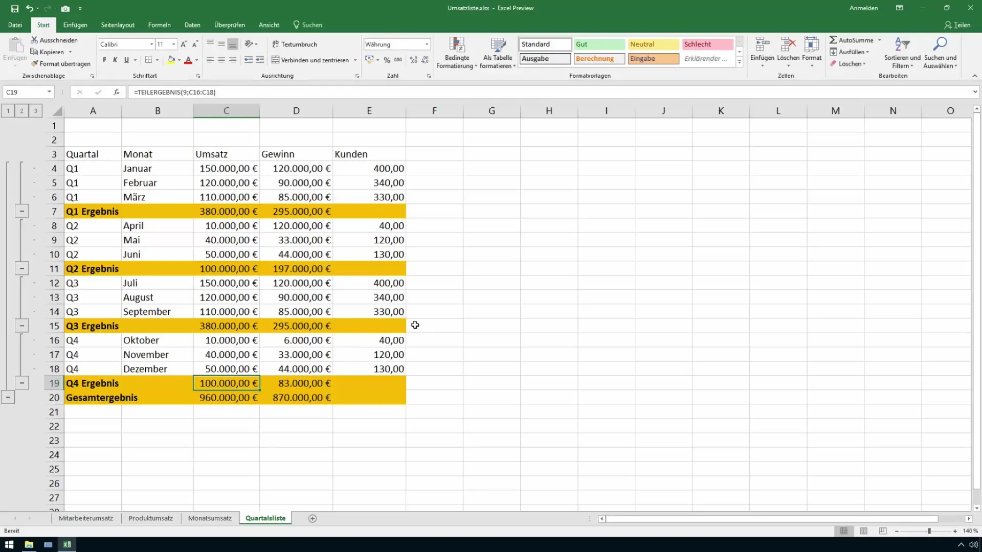
Choose the desired formatting (e.g., orange background color) to highlight the results you have just adjusted. Click "OK" to apply the new formatting.
10. Customize the final presentation
If desired, you can further emphasize the overall result by formatting it in bold. This improves readability and directs the eye to the most important metrics.
Summary
In this guide, you have learned how to create automatic subtotals for your sales data in Excel using the Subtotal function. You can group the quarterly values, calculate the totals, and visually format them to present the results clearly and concisely.
Frequently Asked Questions
How can I activate the subtotal function?You can find the subtotal function in the "Data" tab under the "Outline" section.
What happens when I group by months?Grouping by months results in only one row per month, which does not provide the desired subtotals.
Can I change the formatting of the subtotals at any time?Yes, the conditional formatting can be adjusted at any time to highlight or modify results.
Do I need to manually update the subtotals?No, the subtotals are automatically updated when you change the underlying data.
How can I better highlight the key results?You can use conditional formatting to make changes in color or font size, improving visibility.


