Comparison of two Excel tables

Excel is a powerful tool that allows you to manage and analyze data efficiently. However, it can be challenging to compare multiple tables and identify differences, especially in the fields of controlling and sales. This guide will show you how to compare two Excel tables to ensure that the article numbers in both lists match. We will do this using conditional formatting.

Main Takeaways

• You can compare two tables in Excel to identify deviations in article numbers.
• Conditional formatting allows you to visually highlight differences.
• Excel helps you quickly identify and correct errors such as transposed numbers.

Step-by-Step Guide

Start Excel to open your list of articles and the comparison table. You should have the table ready from which you want to align the article numbers. It is helpful to have this prepared in advance so you can start comparing quickly.

The first table you are analyzing contains the article numbers and the currently available stock. While this information is important for maintaining data consistency, our focus at the moment is on aligning the article numbers. Make sure the list of articles has been entered correctly and is in the appropriate column.

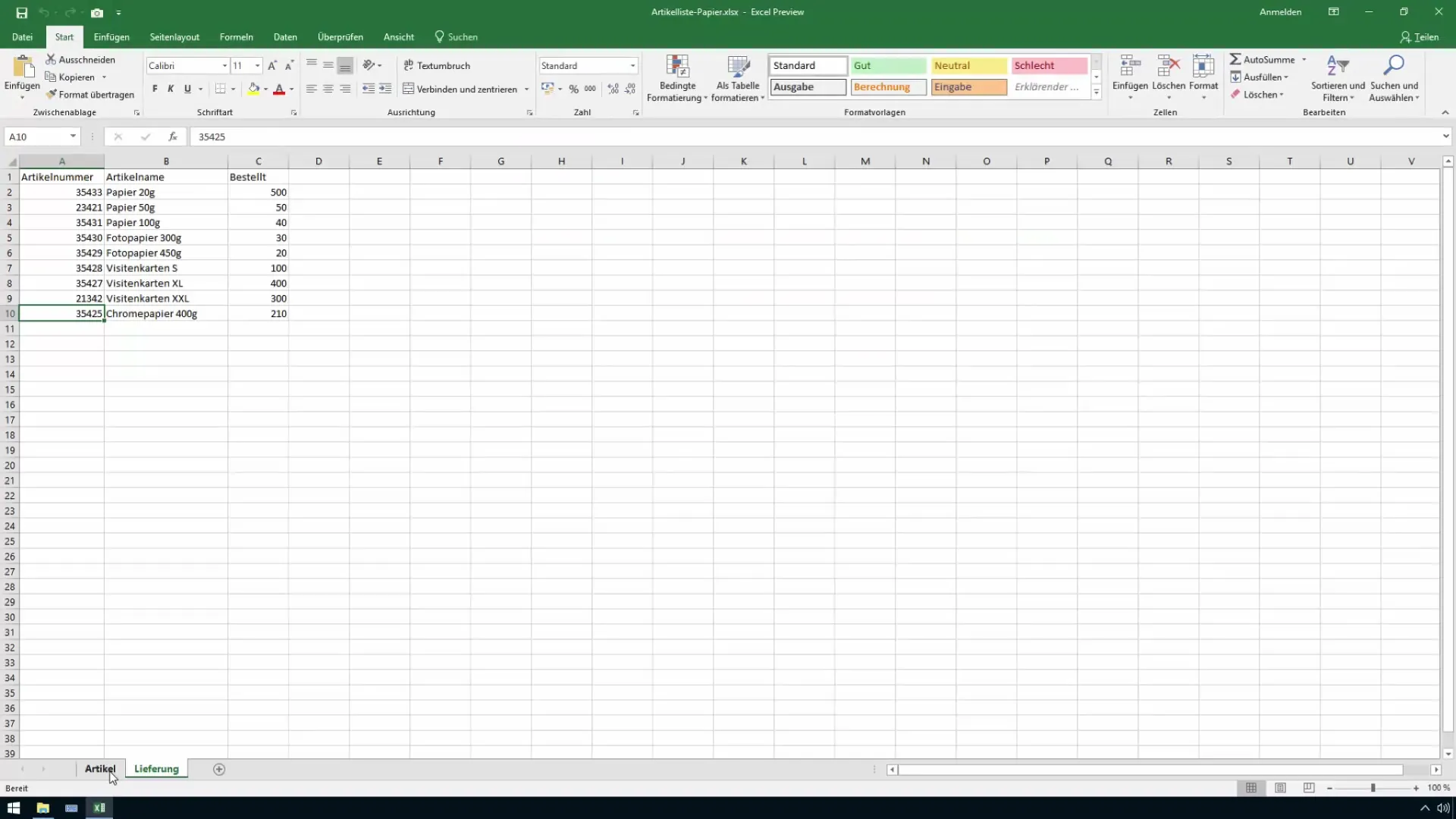
Now, let's focus on how to incorporate the second table for verification. This table should ideally contain the article numbers you want to align. Ensure that both tables are well-structured and understandable so you can easily identify the differences.

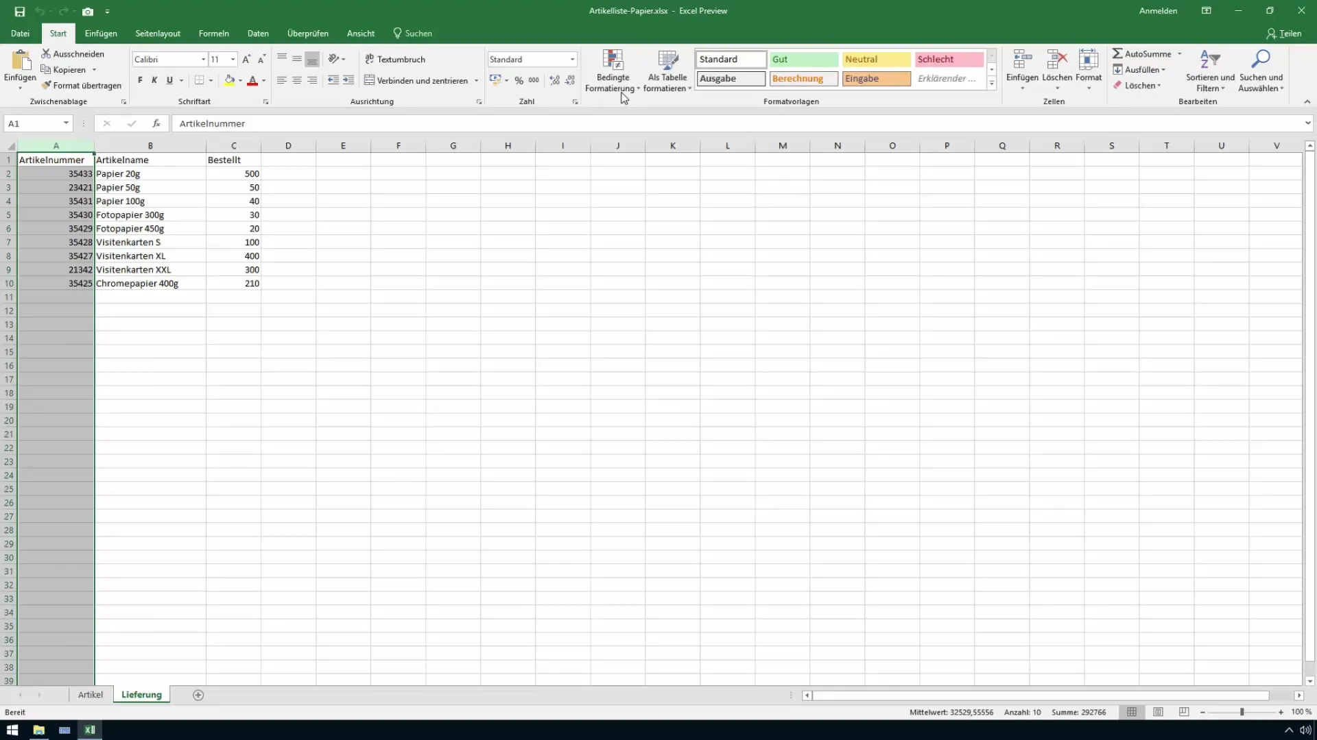
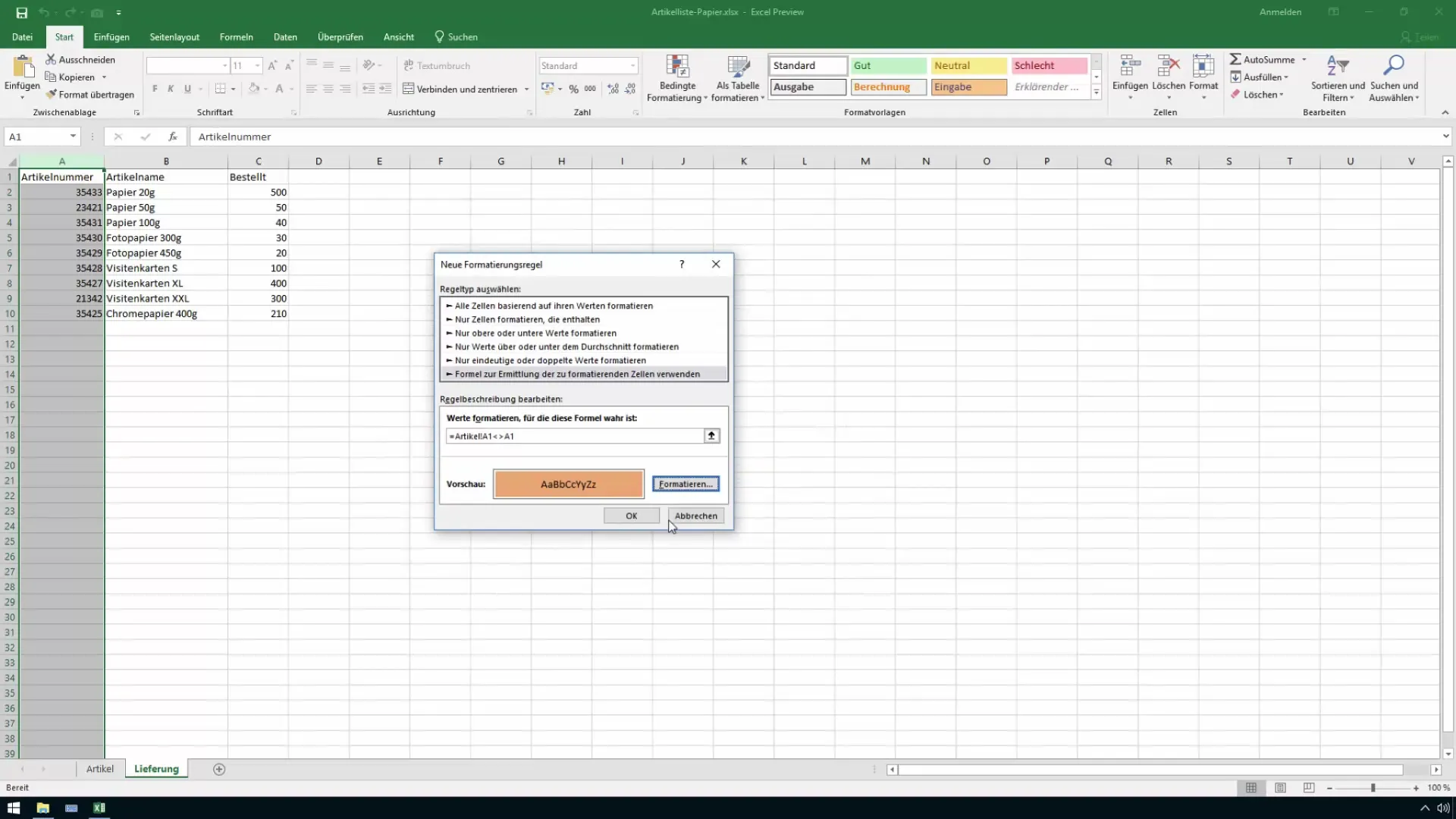
To check if the article numbers match, go back to the first table. Select the entire column A containing the article numbers. Then, open the "Home" menu and select "Conditional Formatting." Here, you can create a new rule to define your comparison environment.

When creating a new rule, you have the option to create a formula to determine differences. You specify that you want to use the values of the article numbers from the other table as your comparison basis.

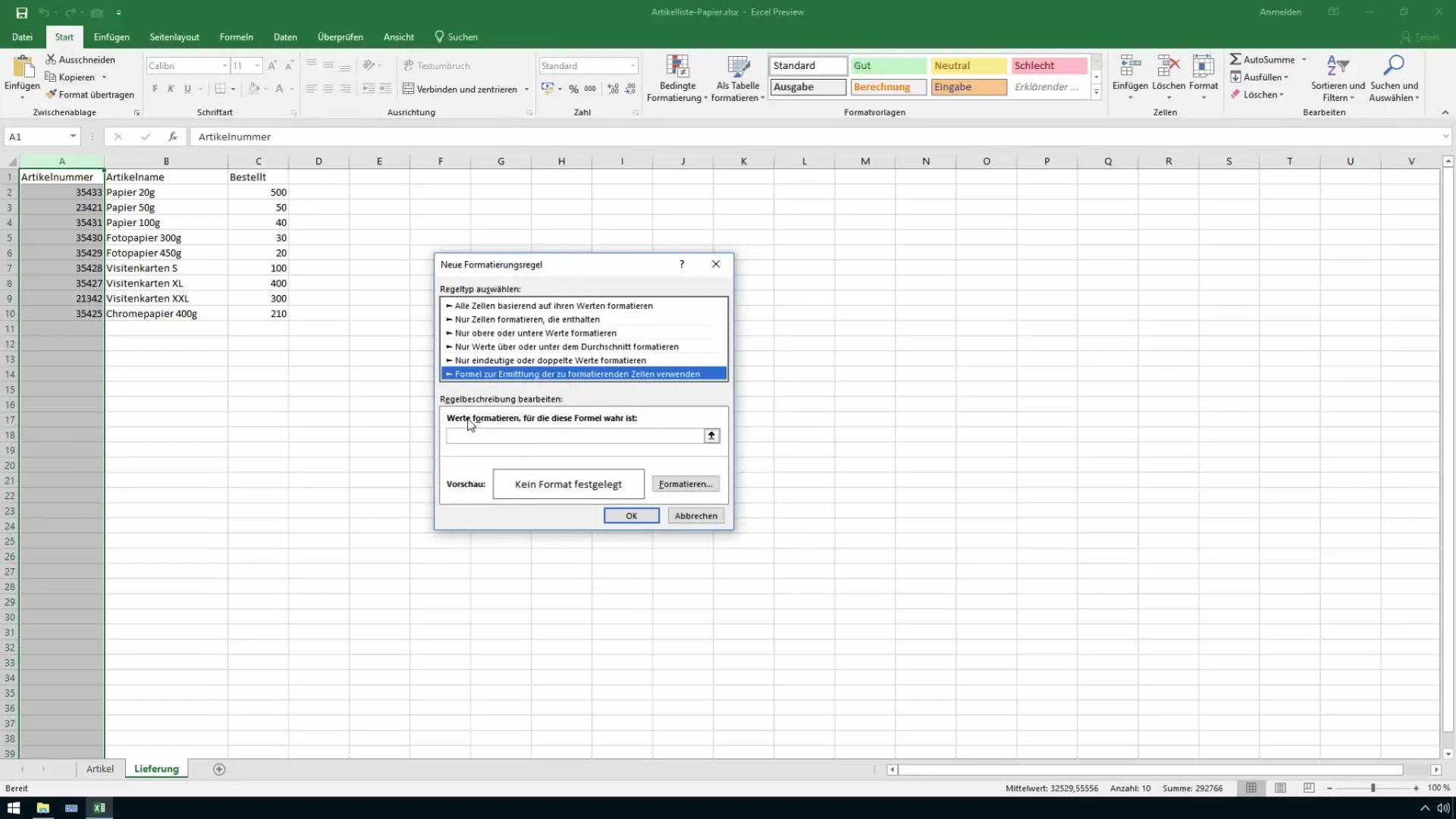
Ensure that you correctly select the range of the list of articles. Start from the top and go through the entire list. Excel will now automatically establish a reference to the data in the other table.

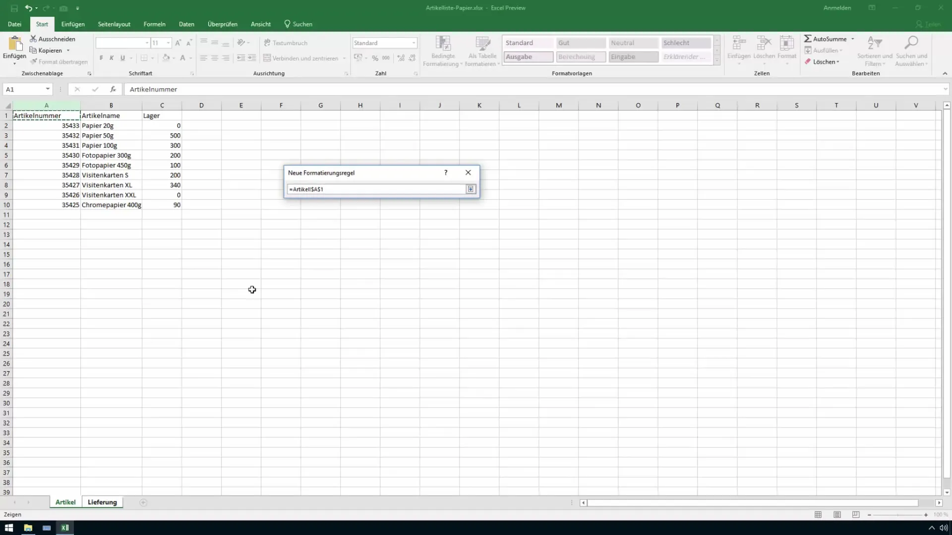
Also, make sure the reference is relative. Therefore, remove the dollar signs so Excel can adjust the formula to each row. You can do this by using the F4 key to switch between reference types until you reach a relative reference without dollar signs.

Once the references are set correctly, you can establish the condition for which article numbers should be marked as different. Add a "less than" or "greater than" sign depending on what you want to compare.

Now that all settings have been made, confirm your rule. The next step is to highlight the differences in color so that incorrect or deviating article numbers stand out immediately.

After applying conditional formatting, you will immediately see which article numbers are different. You will likely notice some errors, such as transposed numbers, which can be easily overlooked.

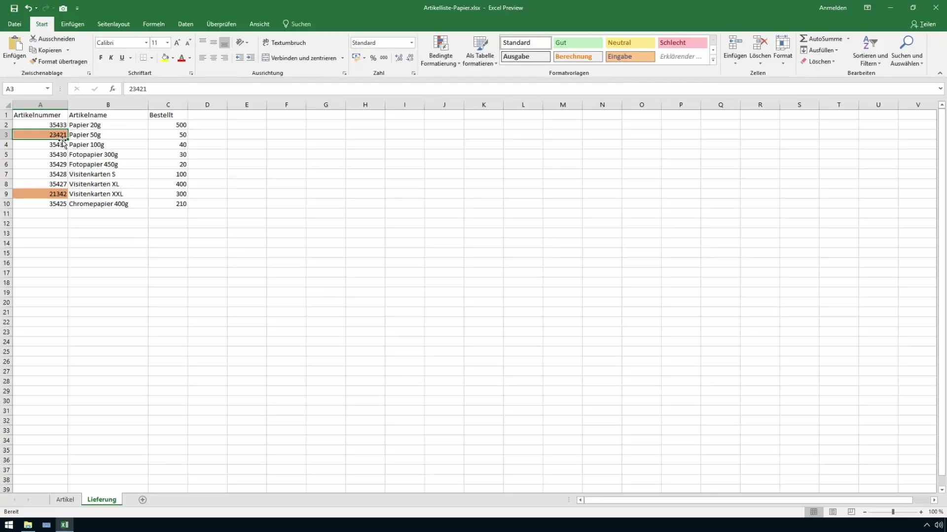
For example, the article number 23421 may have been entered accidentally instead of 23412. Excel will automatically highlight these differences, allowing you to quickly identify and correct them in the list.

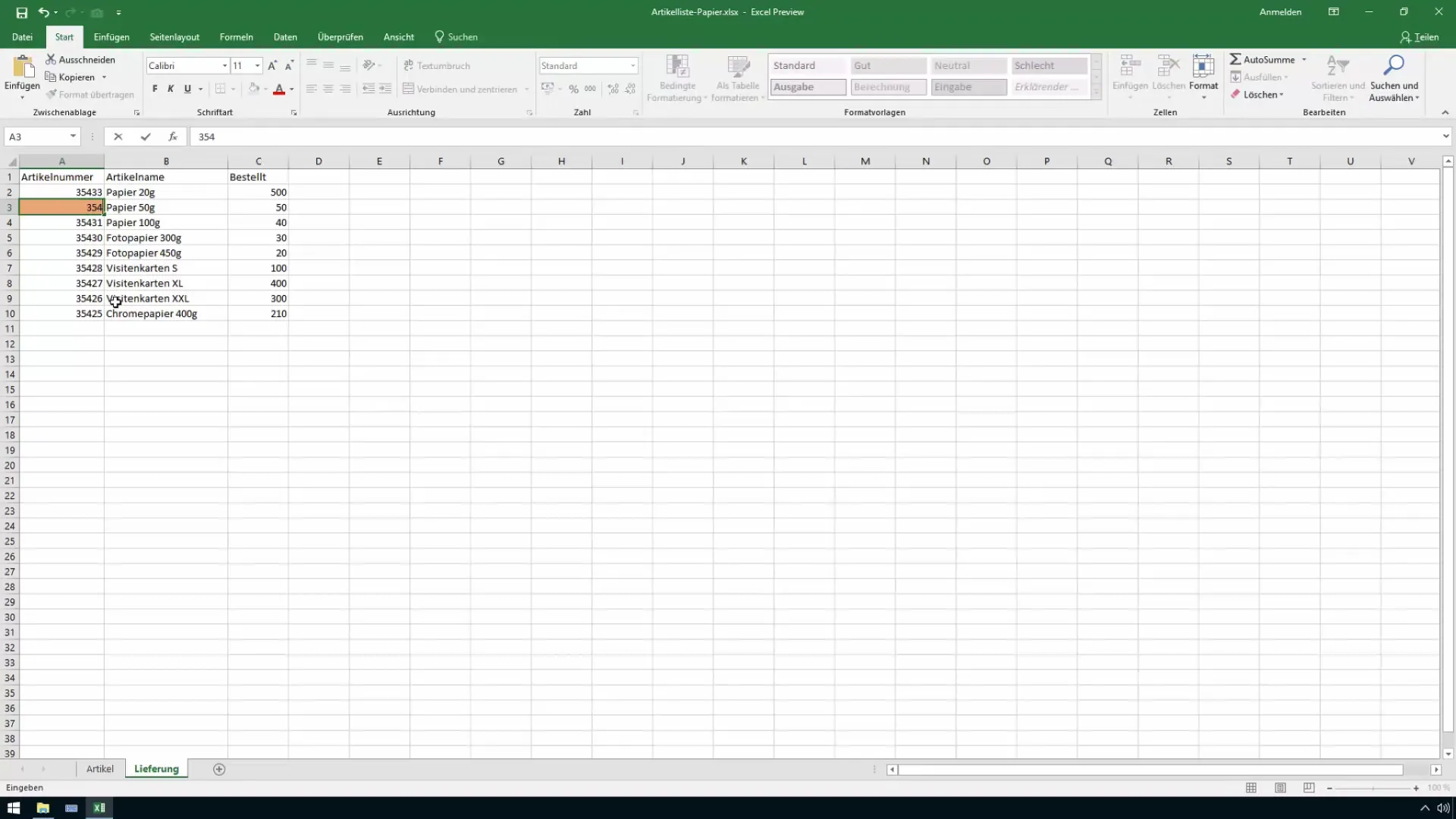
Each time you enter a wrong number, the difference will be displayed immediately. This is extremely helpful in avoiding prolonged work and identifying mistakes in a timely manner.

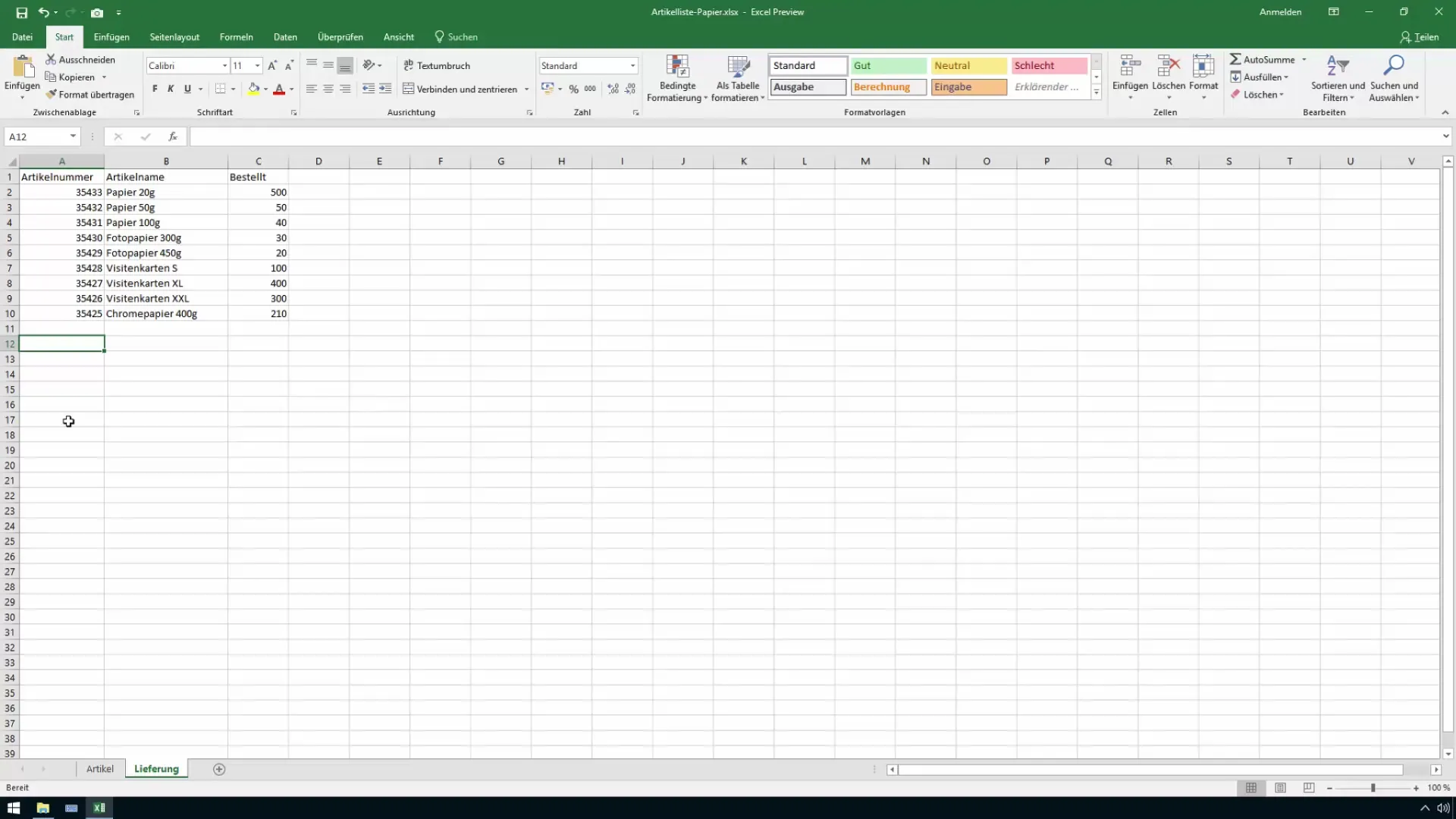
In summary, it can be said that with these simple steps you can implement an effective method for comparing Excel tables. This not only helps with matching article numbers, but can also be applied to article names and other data, making your workday much easier.

Summary

With the methods described, you can efficiently identify differences between two Excel tables. By using conditional formatting, discrepancies are quickly visible, helping you to promptly correct errors or typos and ensure data quality.