Comparing values in Excel

Comparing values in Excel provides you with an effective way to ensure consistency and accuracy in your data. Particularly in controlling and sales, it is important to know whether certain values are present in a reference table. In this guide, you will learn step by step how to perform these comparisons in Excel. You will see how to apply the corresponding formulas and how to highlight differences visually.

Key Takeaways

• You can use the comparison formula in Excel to check if a value exists in a reference table.
• Conditional formatting helps you to visually represent matches and discrepancies in color.
• The comparison is not only useful for item numbers or names, but can be applied to different data fields.

Step-by-Step Guide

To compare values in a reference table, you first need an item list and a reference table. Below, I will explain the entire process of value checking in Excel.

Step 1: Create and Prepare Tables

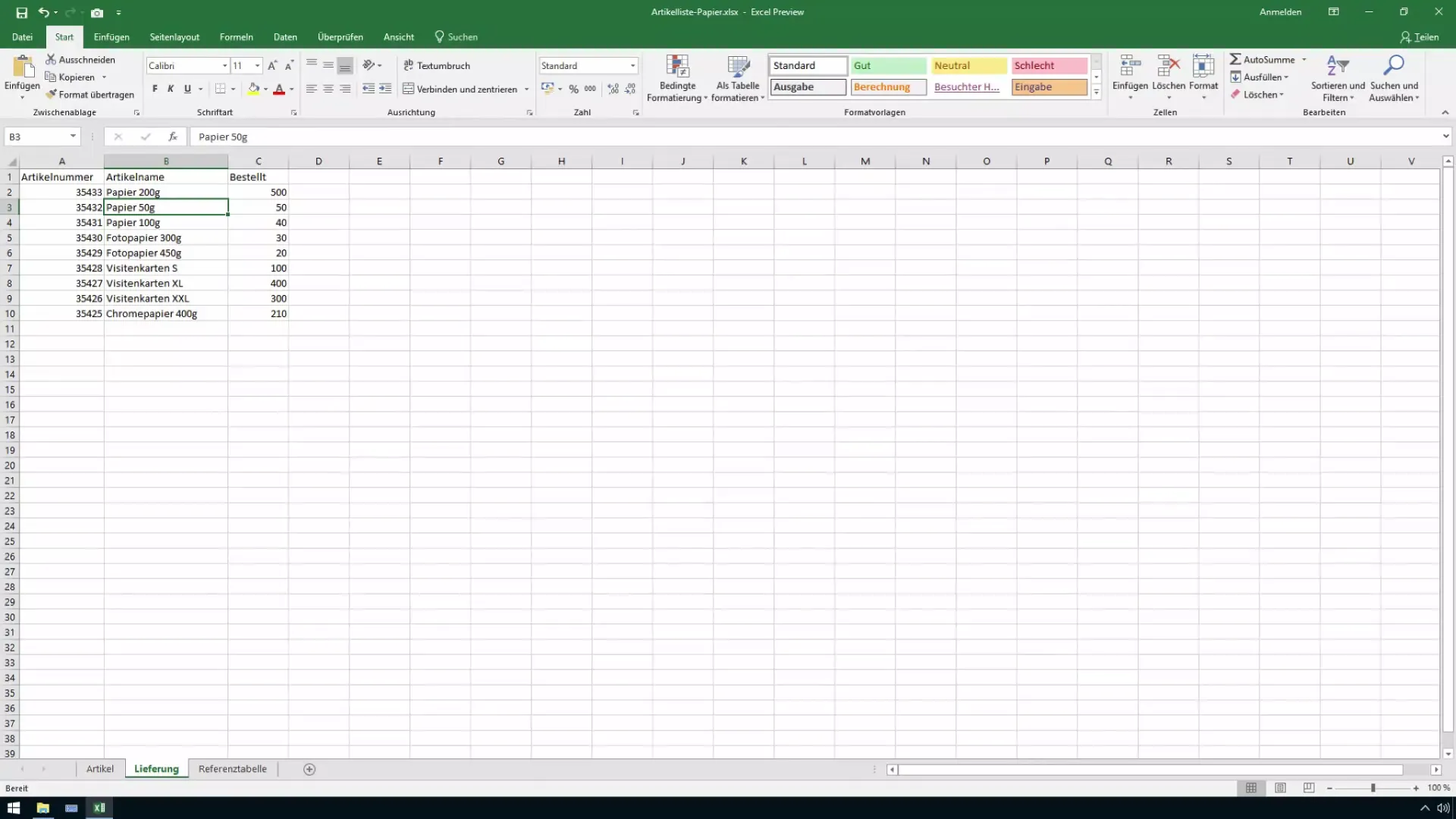
First, create your item list and reference table in an Excel document. The item list should contain all relevant item information, such as the names and quantities of your products. The reference table is a long list of all items you want to compare with your item list.

Step 2: Insert Comparison Formula

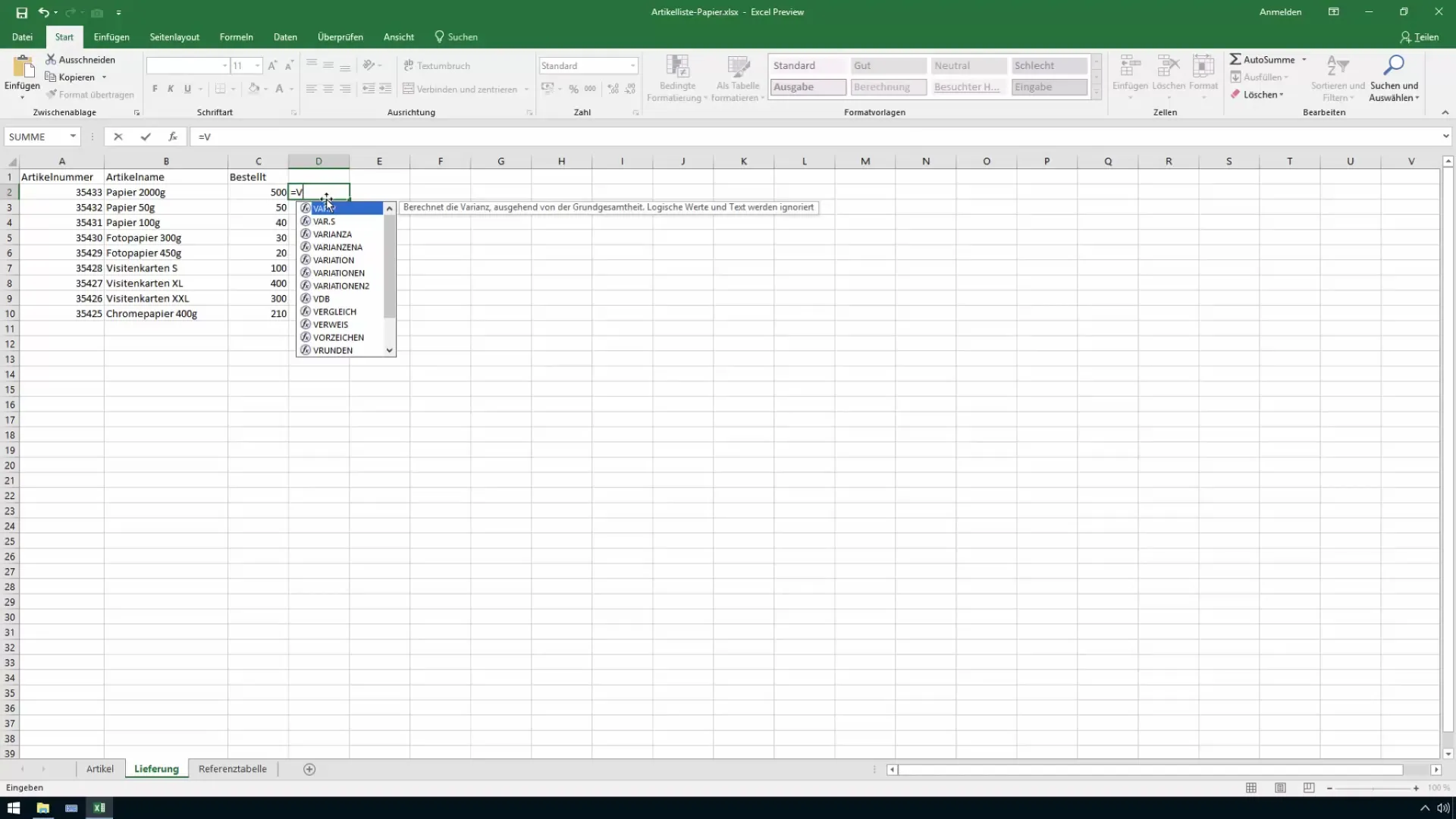
Now it's time to create the comparison formula. You insert the formula =MATCH(lookup_value,lookup_array,match_type) into the cell where you want to see the comparison result. The lookup_value is the item you are searching for. In our case, it could be a specific paper like "Paper 200 g".

Step 3: Define Lookup Array

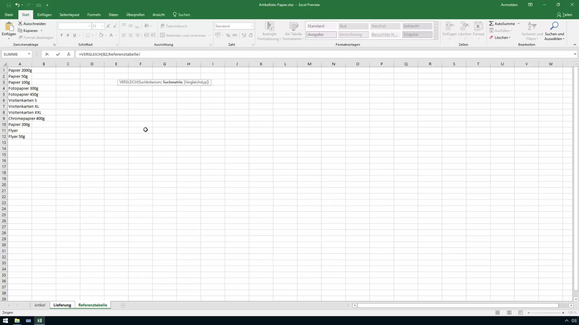
The lookup array is your reference table containing the values you want to compare. To work accurately, select the entire column of your reference table that contains the item names. Ensure that the reference table is properly prepared to ensure accurate comparisons.

Step 4: Specify Match Type

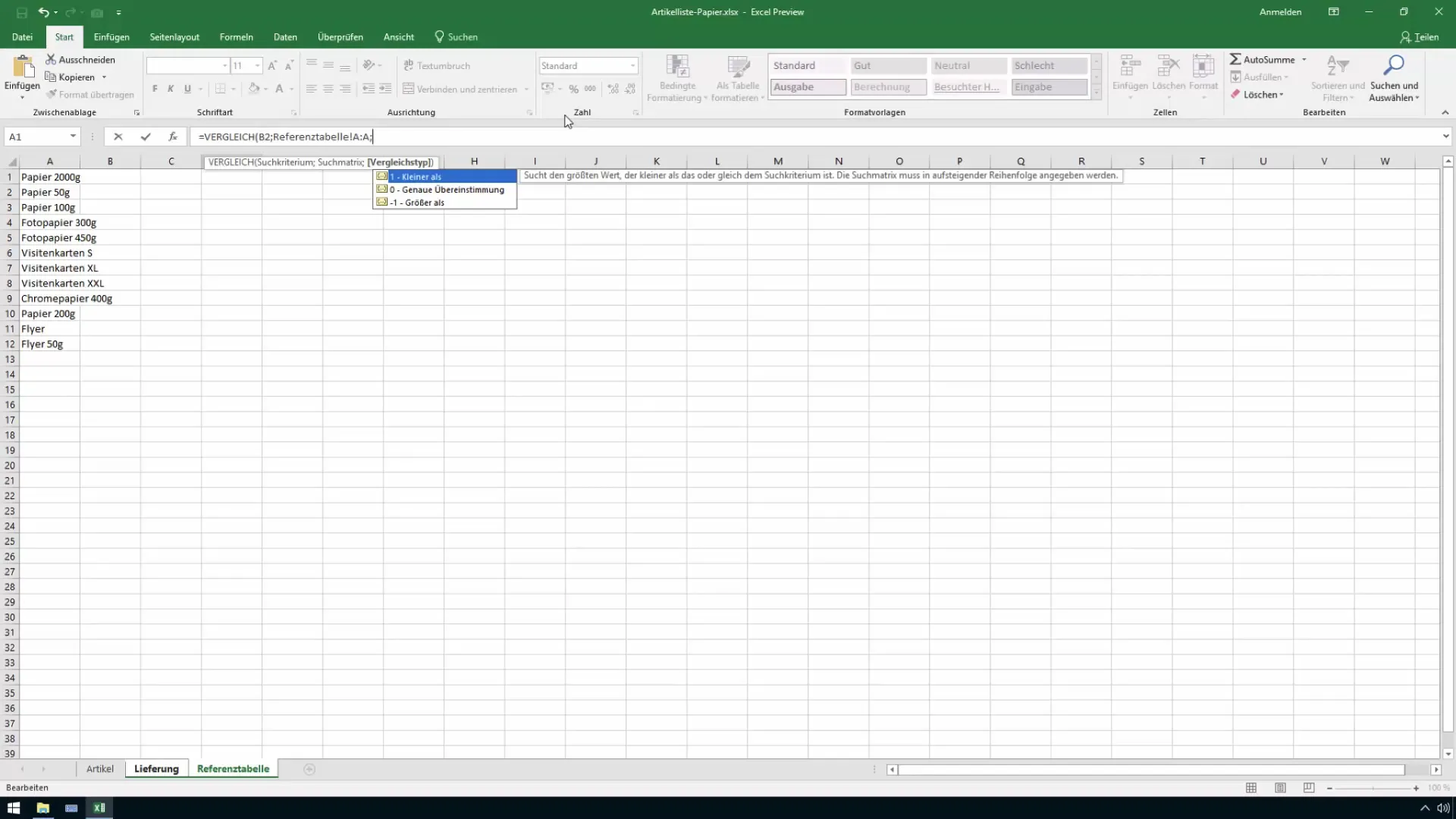
In the next step, specify the match type. Here, use the value 0 (zero) for an exact match. This setting ensures that only identical values are recognized as matches, which is important for your project.

Step 5: Verify Results

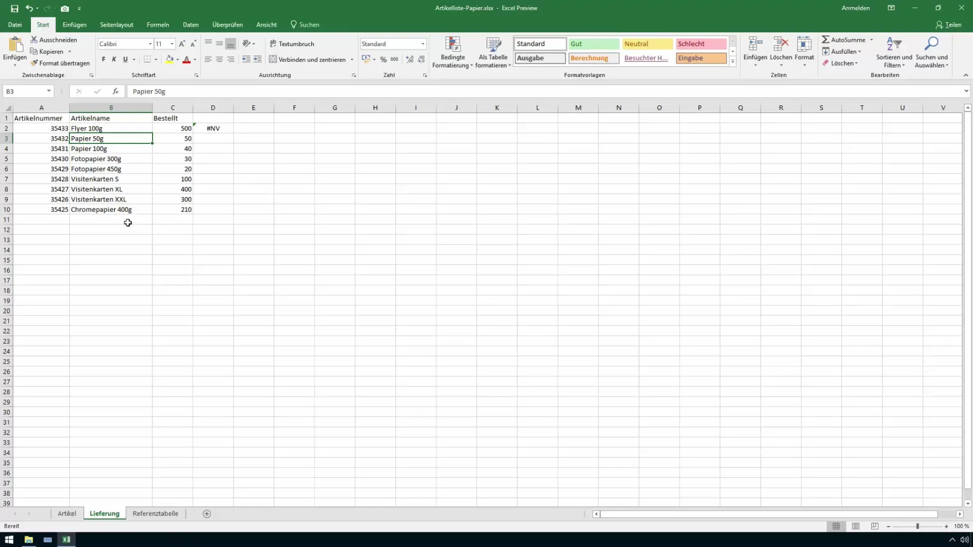
After applying the formula, you should verify the results in the cell. If the value is present, Excel shows the position in the reference table. If the value is not found, Excel displays an error such as "NA".

Step 6: Utilize Conditional Formatting

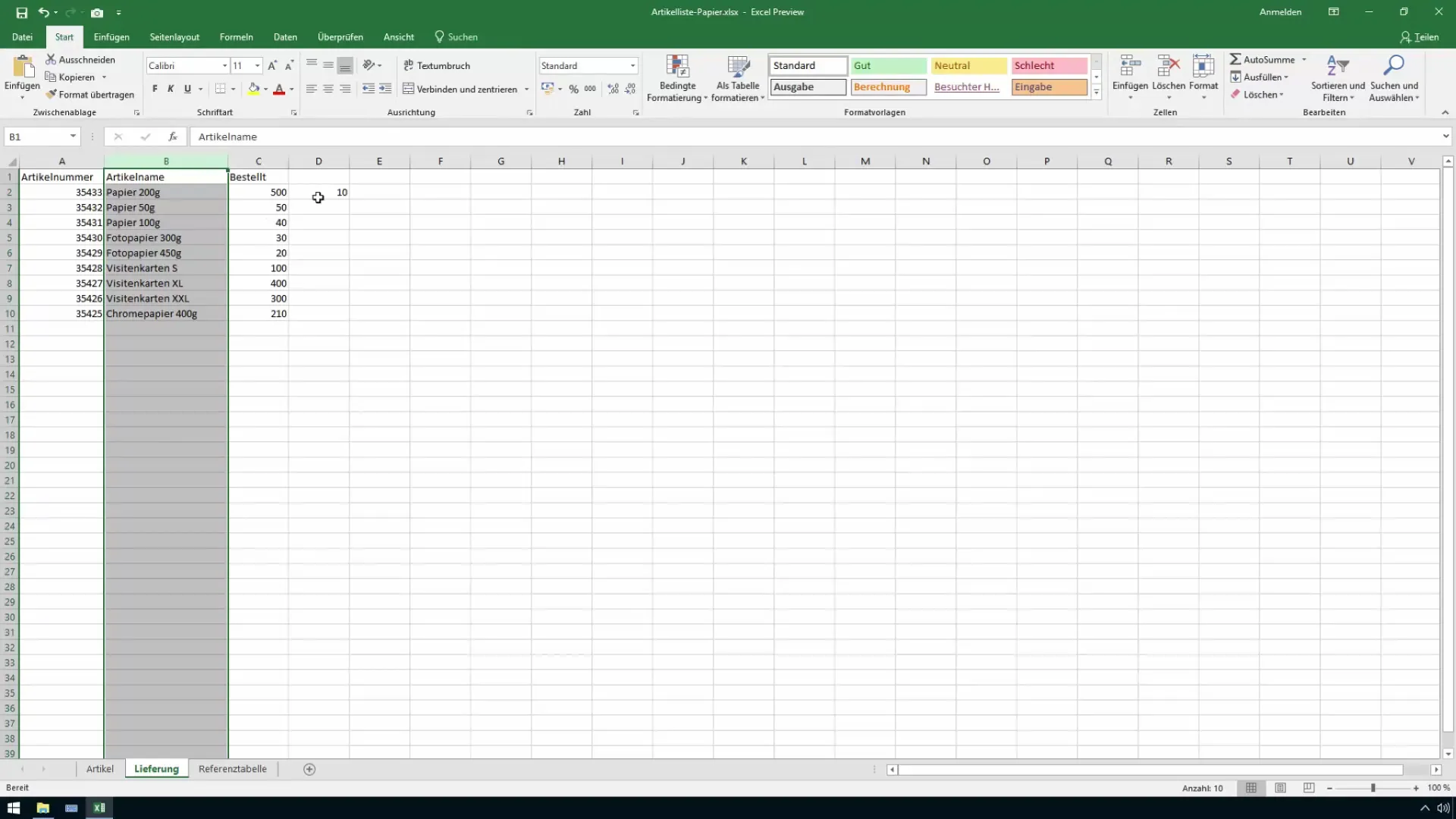
To make visual statements about the found values, you can use conditional formatting. Highlight the column where the comparison results appear and click on "Conditional Formatting." There, you can create new rules to, for example, mark non-found values in red.

Step 7: Review Comparison Results at a Glance

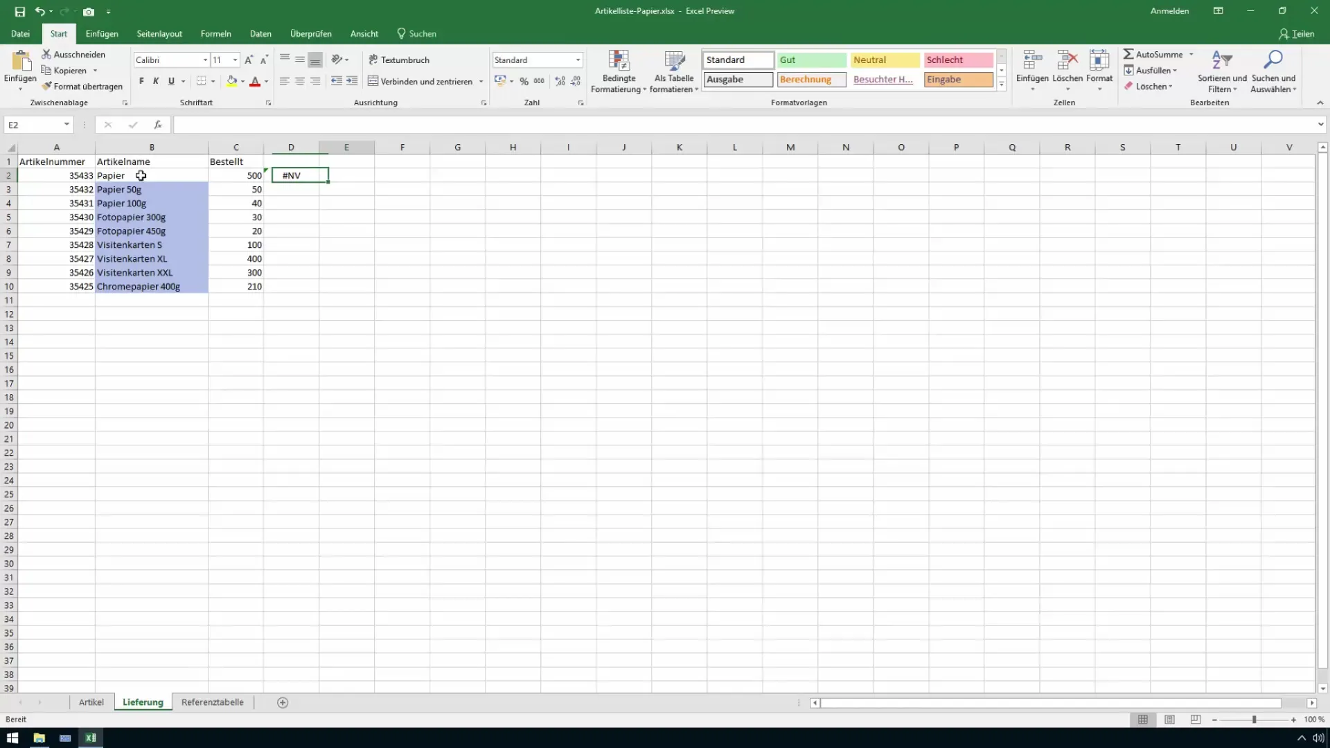
After setting up conditional formatting, you can easily review the results. If a value is not present in the reference table, this will be displayed accordingly. You can also make further adjustments, such as bolding the font or choosing different colors to enhance clarity.

Step 8: Test Different Values

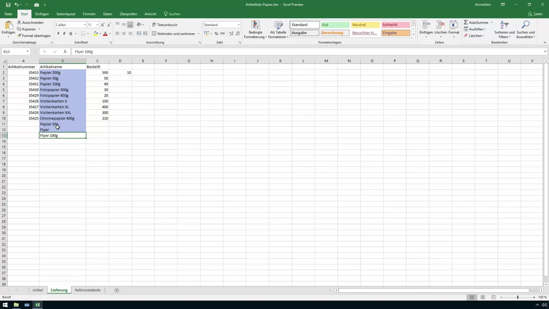
Now you have the opportunity to test different items. Simply enter new values in the search field to see if they are included in the reference table. This functionality helps you to promptly identify changes or errors in your data.

Step 9: Documentation and Feedback

It is important to document the work and clarify any questions. Use the comment field in Excel to leave notes or to communicate with colleagues about the discrepancies found. This will make the process even smoother.

Summary

Comparing values in a reference table helps you identify errors and ensure the accuracy of your data. By using comparison formulas and conditional formatting in Excel, you can efficiently monitor whether the items you are looking for are present.