Detect and highlight duplicate values in Excel

Duplicate values in Excel can lead to confusion and waste valuable time. When working with large amounts of data, it is often difficult to keep track, especially when there are many similar or identical entries. This guide shows you how to quickly and effectively identify and highlight duplicate values in your Excel table.

Key Takeaways

• You can choose different colors for highlighting duplicate values.
• Changes to entered values immediately affect the highlighting.
• Using conditional formatting is a straightforward method for identifying duplicate values.

Step-by-Step Guide

To highlight duplicate values in your Excel table with colors, follow these simple steps:

First, open your Excel table containing the data you are working with. In this example, we are using the paper product list. To highlight the desired values accordingly, navigate to the reference table where the relevant entries are located.

After opening the table, you should get an overview of the entries. In a long list, it can be easy to lose track. For example, there are two entries for "Paper 50 g," which may not be immediately noticeable in an extensive list. To make these duplicate values visible, it is important to follow the next steps.

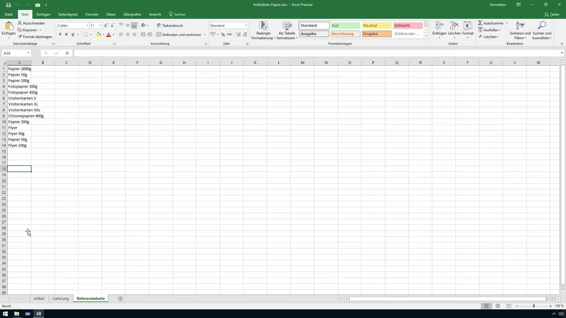
Now, select the cell or range you want to analyze. For example, you can highlight the entire column to have all duplicate entries in view. To make it easier to select, you can enlarge the range so you can see better what you are doing.

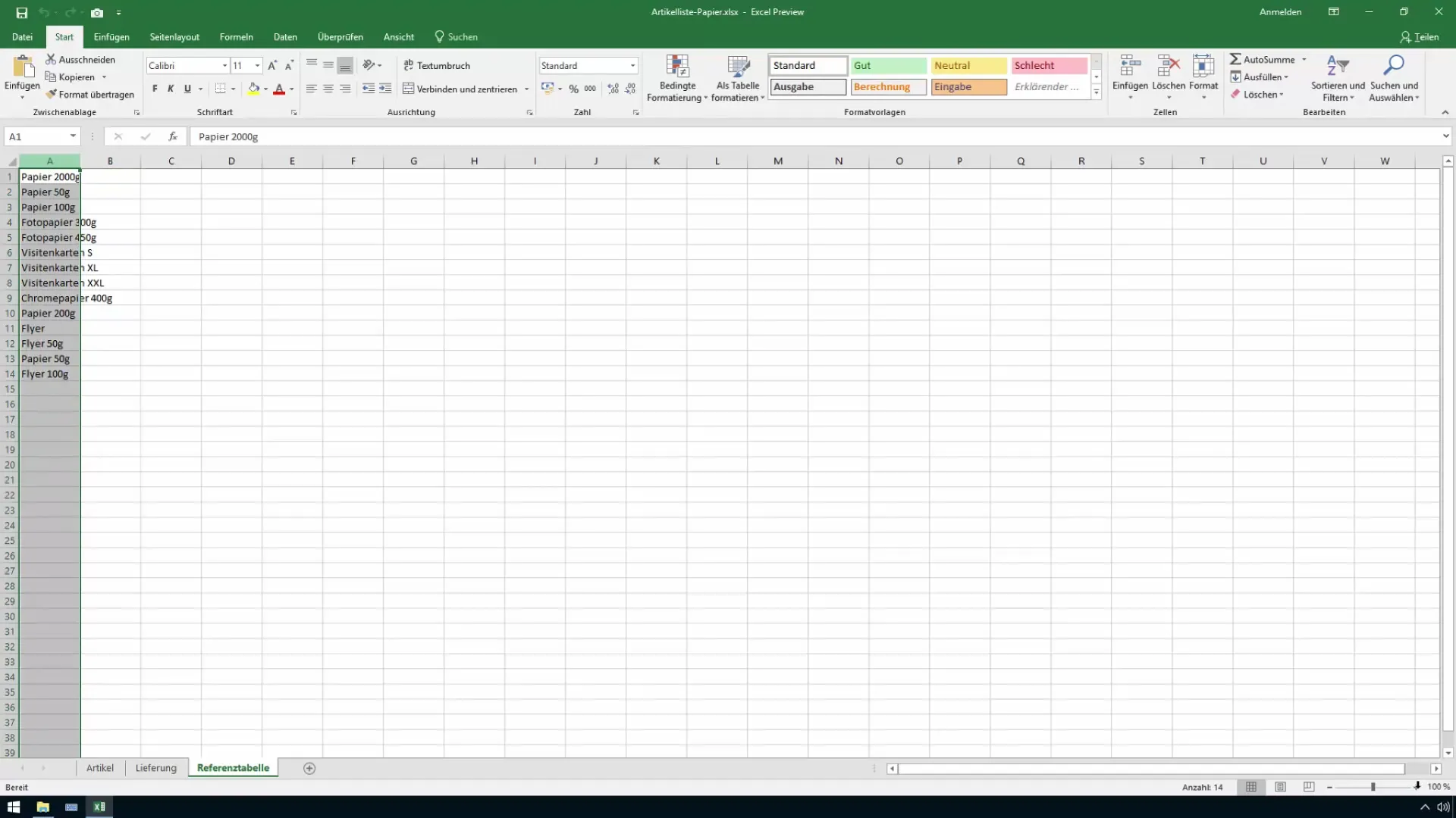
Now go to the "Home" tab. Here, in the "Styles" group, you will find the "Conditional Formatting" option. This method is particularly useful for making visual distinctions in your data. Click on "Conditional Formatting."

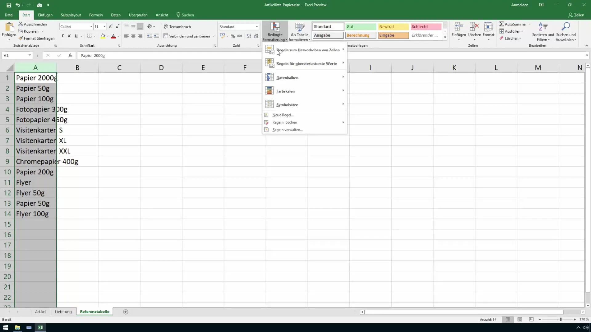
In the menu that opens, select "Highlight Cells Rules." This will open a selection of options for formatting your cells. Look for "Duplicate Values" in the list of options.

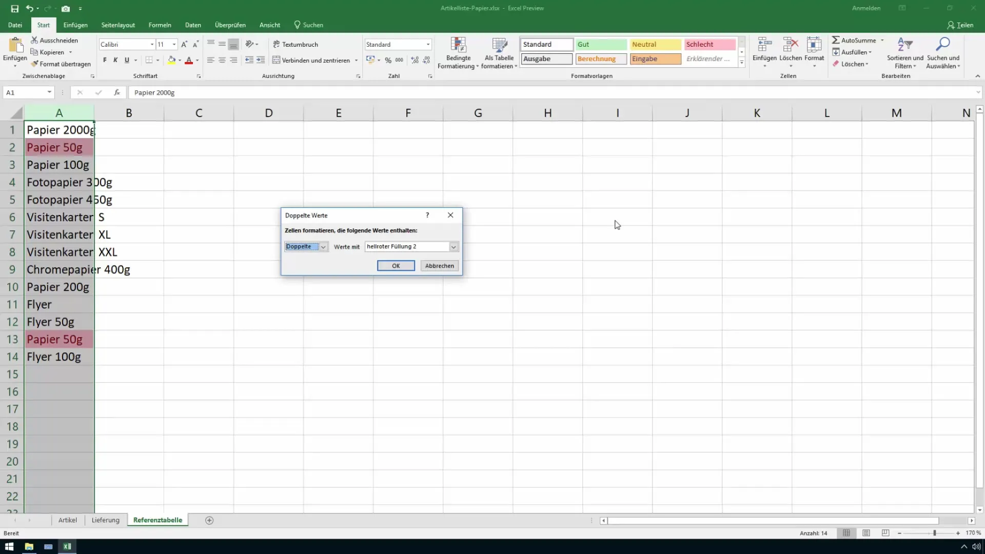
Now you can choose the format for highlighting the duplicate values. You have the option to select different colors like light red, yellow, green, or other fill colors. Choose the desired color and then click "OK" to confirm your selection.

After confirming, you will see that all duplicate values in your table are now highlighted in color. This visual support helps you immediately identify all duplicate entries at a glance. For example, looking at the list, you will see if "Paper 50 g" is present multiple times.

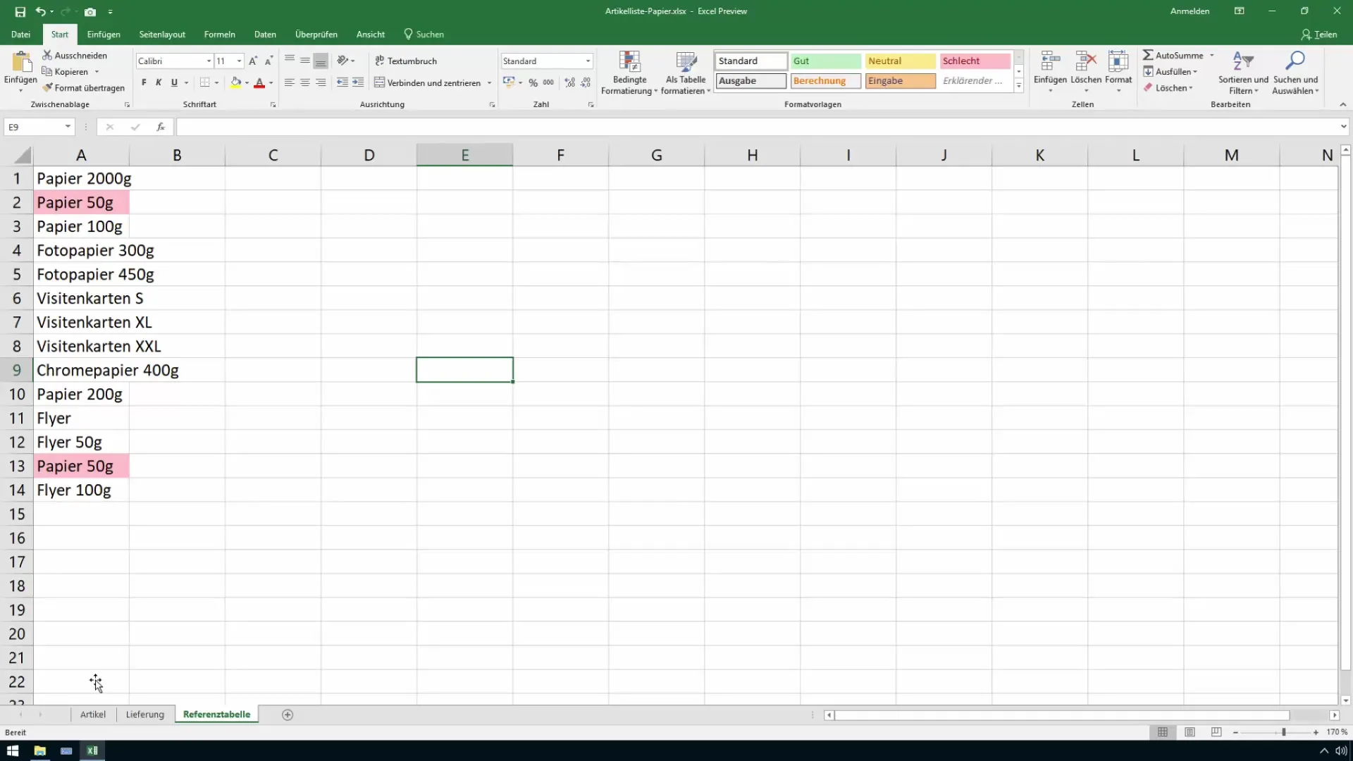
If you now change one of the cells, for example, to "500 g paper," the color highlighting will be automatically removed as the entry is now unique. This way, the list remains up-to-date without manual intervention.

You can also add more entries or edit existing ones. If you see a new duplicate value like "Flyer" has appeared, you can immediately identify and potentially edit or remove it.

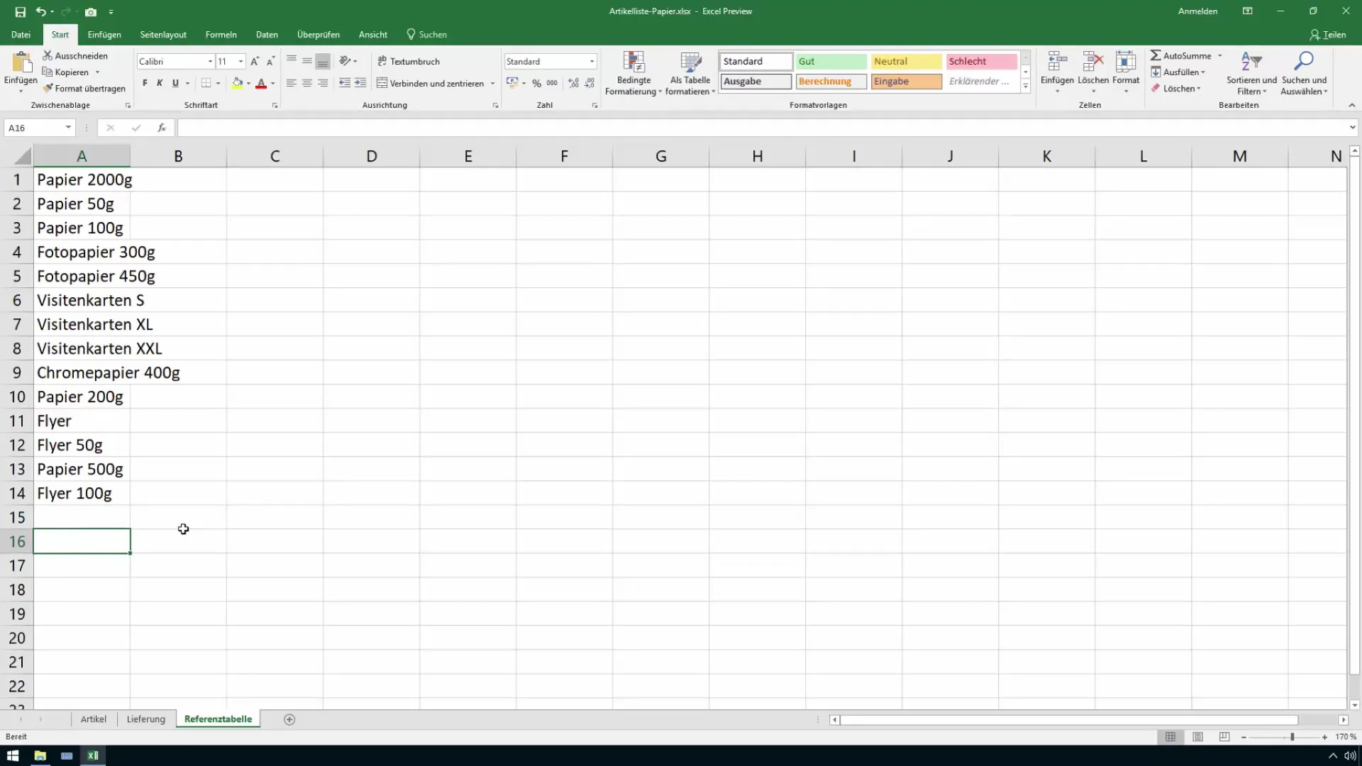
This is how efficiently highlighting duplicate values in Excel is possible. You can adjust your data at any time, and the highlights will reflect these changes immediately. If you have any questions or want to clarify further aspects of using Excel, feel free to ask in the comments.

Summary

In this guide, you have learned how to quickly and easily highlight duplicate values in an Excel table with colors. With the method of conditional formatting, you keep track and immediately recognize where there are duplicate entries.