Format cells in Excel effectively with color coding

Excel can do much more than just simple calculations. One of the useful functions you can use in your Excel work is cell color formatting. This allows you to make information visually appealing and highlight important data immediately. Below I will explain to you specifically how to perform color code formatting in Excel.

Main Takeaways

• You can format cells in Excel with specific colors to highlight information.
• The color code table helps you choose the correct color numbers for your cells.
• Using square brackets to enter the color number is crucial for formatting.

Step-by-Step Guide to Color Code Formatting

Using the Color Code Table

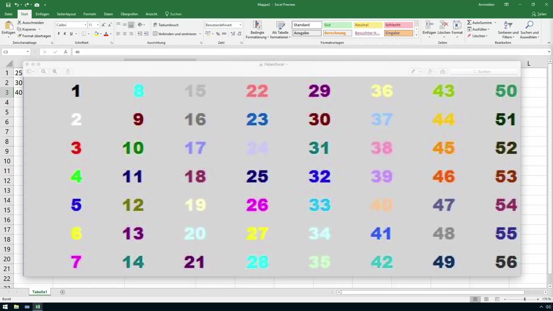
Before you can start formatting, it is important to have an understanding of the color code table in Excel. This table contains the color numbers that you can use to apply specific colors. For example, the number 32 represents a deep blue and the number 44 represents a yellow. So, if you want to select a color, you should have the corresponding number ready.

Selecting Cells

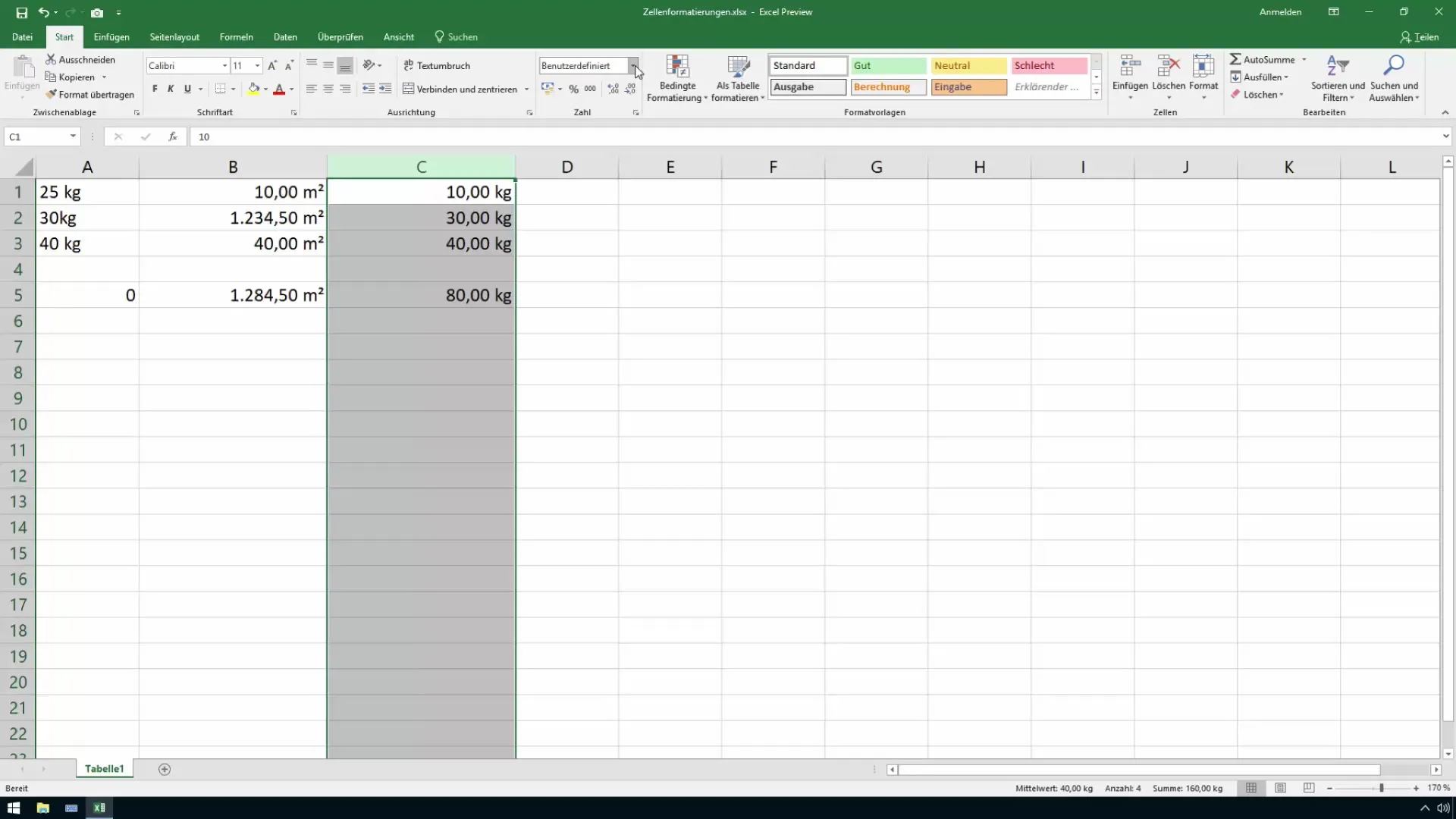
To apply the desired formatting, first select the cells you want to format. In this example, we will use column C. Highlight the cells to which you want to assign a color.

Opening Custom Formatting

To perform color code formatting, you need to access Custom Formatting in Excel. Click on "More Number Formats" and select "Custom." This option gives you the flexibility to format your cells by entering color numbers.

Entering Color Number

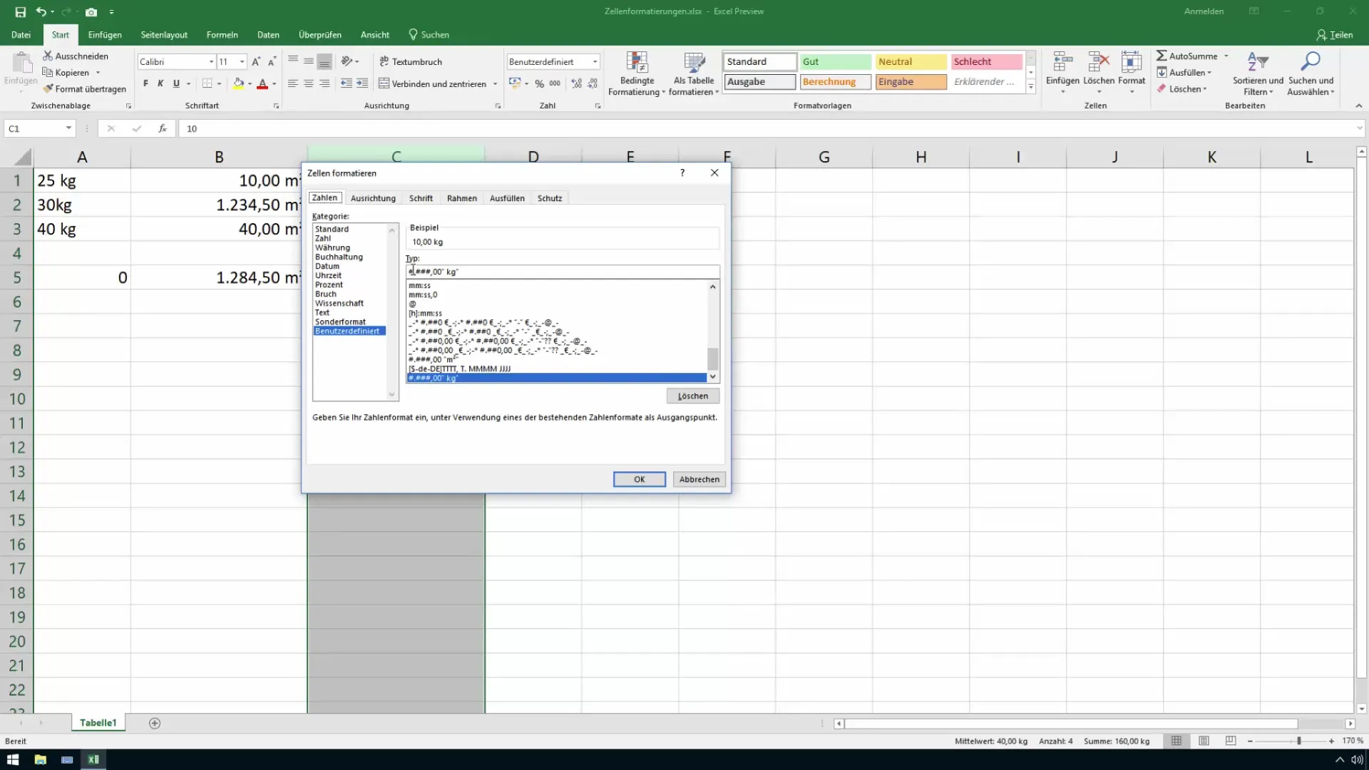
Now comes the exciting part: Enter the color number in the formatting line. To do this, start by entering square brackets: [. Hold down the Alt key and then press 8 and 9 to enter the square brackets "[" and "]". Then enter the number of the desired color. For example, for a deep blue, write [32] and confirm your entry with "OK".

Checking Color Formatting

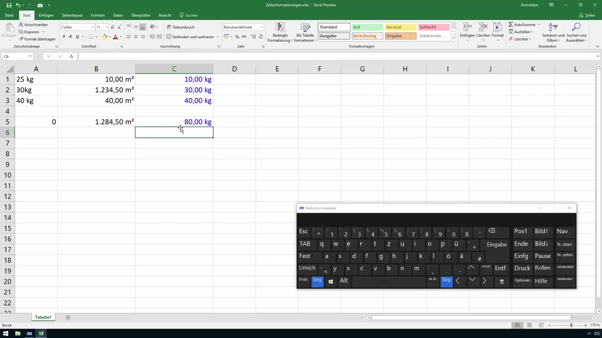
After entering the color number and applying the formatting, you should immediately see how the cells change. In our case, all cells in column C should now appear in a deep blue. Make sure that the terms of the format style are also adjusted accordingly.

Making Color Changes

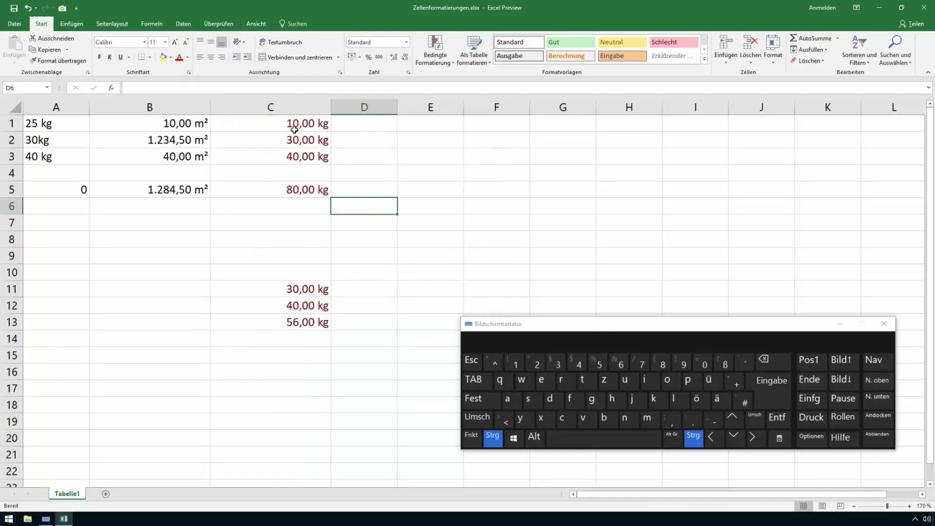
If you want to change the color later, repeat the steps of selecting the cells and opening the Custom Formatting. For a new color, such as dark red, use color 30 and adjust the formatting accordingly. You will see that the shades in the cells update immediately.

Summary

Color code formatting in Excel is an extremely useful tool for visually organizing and highlighting data. By using color numbers and incorporating them into the Custom Format, you can achieve an appealing presentation of your data. Try it out and make your Excel tables shine!