Effectively using VLOOKUP across multiple columns in Excel

Excel is a powerful tool for controlling and sales that helps you process data effectively and perform precise analyses. One of the most common requirements is searching for values across multiple columns. In this guide, you will learn how to use the VLOOKUP function in Excel to match sales figures and inventory levels using the item number, product name, and warehouse. This can help you automate processes and save time.

Main Insights

• The VLOOKUP can be applied across multiple criteria.
• Combining functions like INDEX and SUMPRODUCT allows for flexible data analysis.
• Array formulas provide a more efficient alternative to traditional VLOOKUP approaches.

Step-by-Step Guide

Step 1: Prepare Your Data

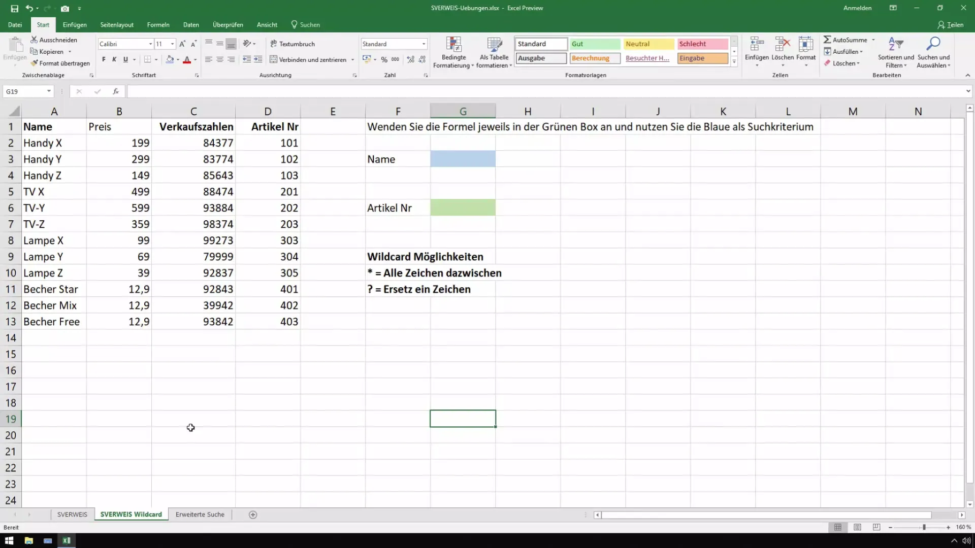
Before working with VLOOKUP, make sure your data is well-structured. Your table should include columns for item number, product name, and inventory level. Prepare your data in a clear format so that you can easily access it later on.

Step 2: VLOOKUP Basics

First, we will use the basic functions to search for values. You will see that this is not limited to a single cell but extends across multiple criteria. A simple VLOOKUP function typically works by entering an item number to find the product name.

Step 3: Initiate Advanced Search

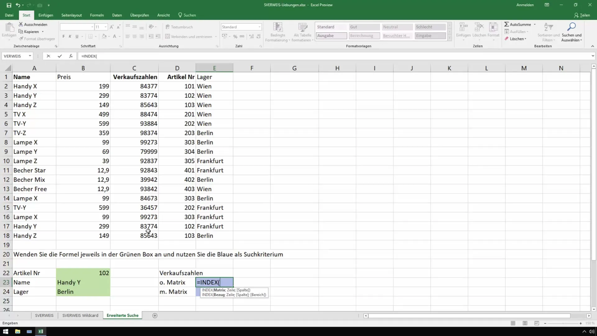
Now, let's implement an advanced search. Suppose you are looking for sales figures for the product "Handy Y." Different warehouse locations may play a role here. To make the search more differentiated, we will use not only the item number but also the inventory level.

Step 4: Use INDEX Function

Now we move on to the INDEX function, which allows you to not only filter out specific values but also search an entire column for the desired values. Select the appropriate range to generate the sales figures.

Step 5: Use SUMPRODUCT for Conditions

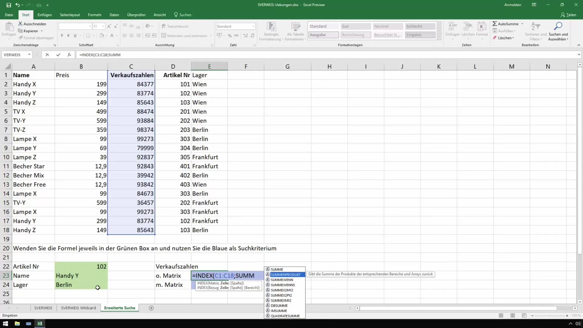
To check multiple conditions simultaneously, we use the SUMPRODUCT function. This function allows you to combine different arrays and perform a total value analysis. Start by defining the different data ranges you want to compare.

Step 6: Define Arrays

Define your arrays to correspond to the data in the respective columns. An array can be a collection of values that are analyzed sequentially. Use the correct brackets to correctly address the different arrays within your formula.

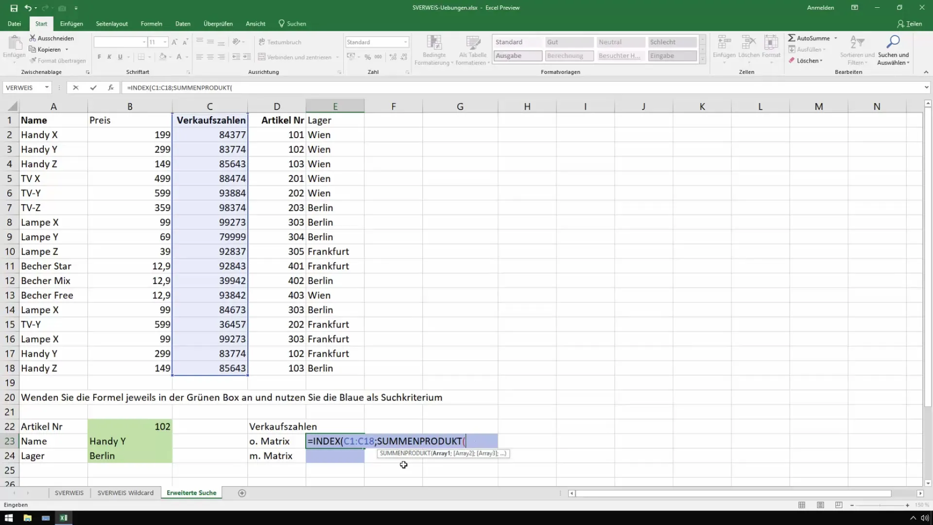
Step 7: Compare Data

This step involves comparing the arrays. You want to ensure that the item numbers, names, and warehouse locations match. This means working with multiplication in the formula to perform the condition checking.

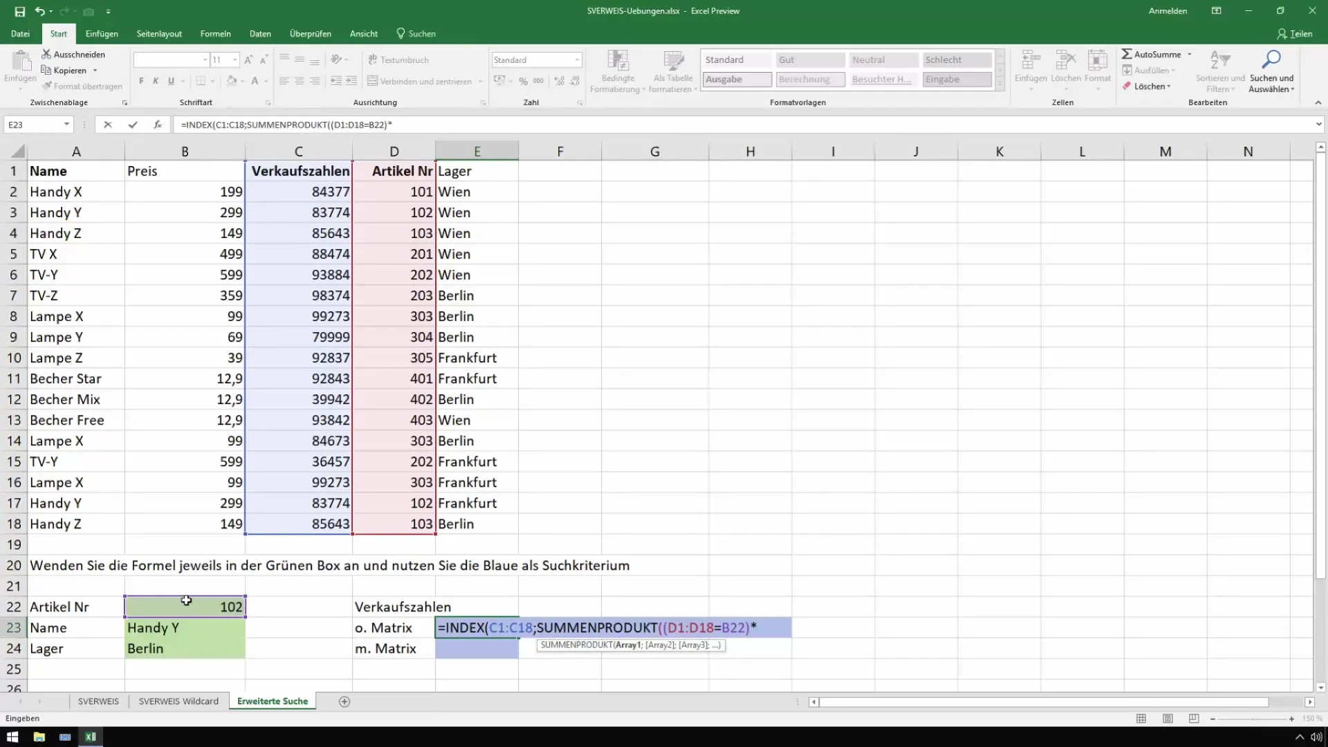
Step 8: Return Correct Result

To get the final result, add a row reference in your formula. By finding a valid entry in the row, you can return the sales figures. Precise bracketing is important for this to work.

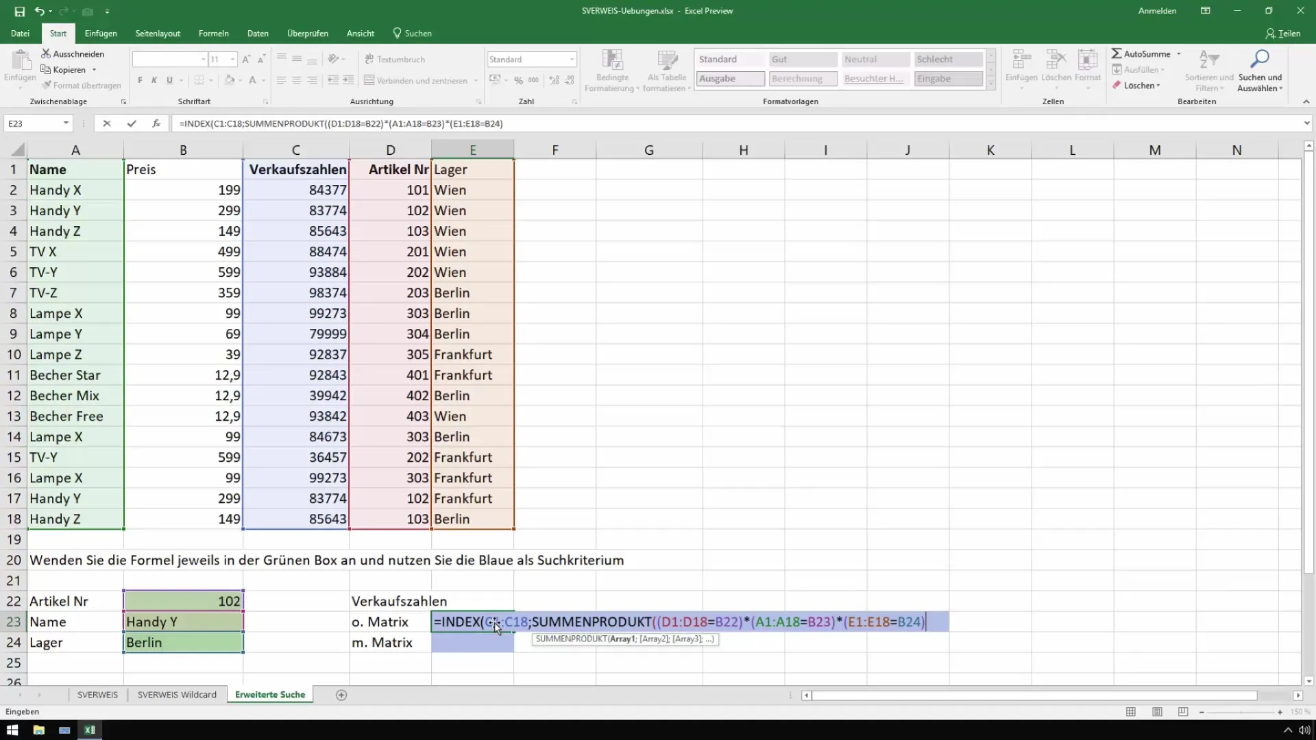
Step 9: Troubleshooting

If your result shows "#VALUE!", it is often because there are no matching entries in the cells you selected. Experiment with different warehouse sets for the item number to clean up the data.

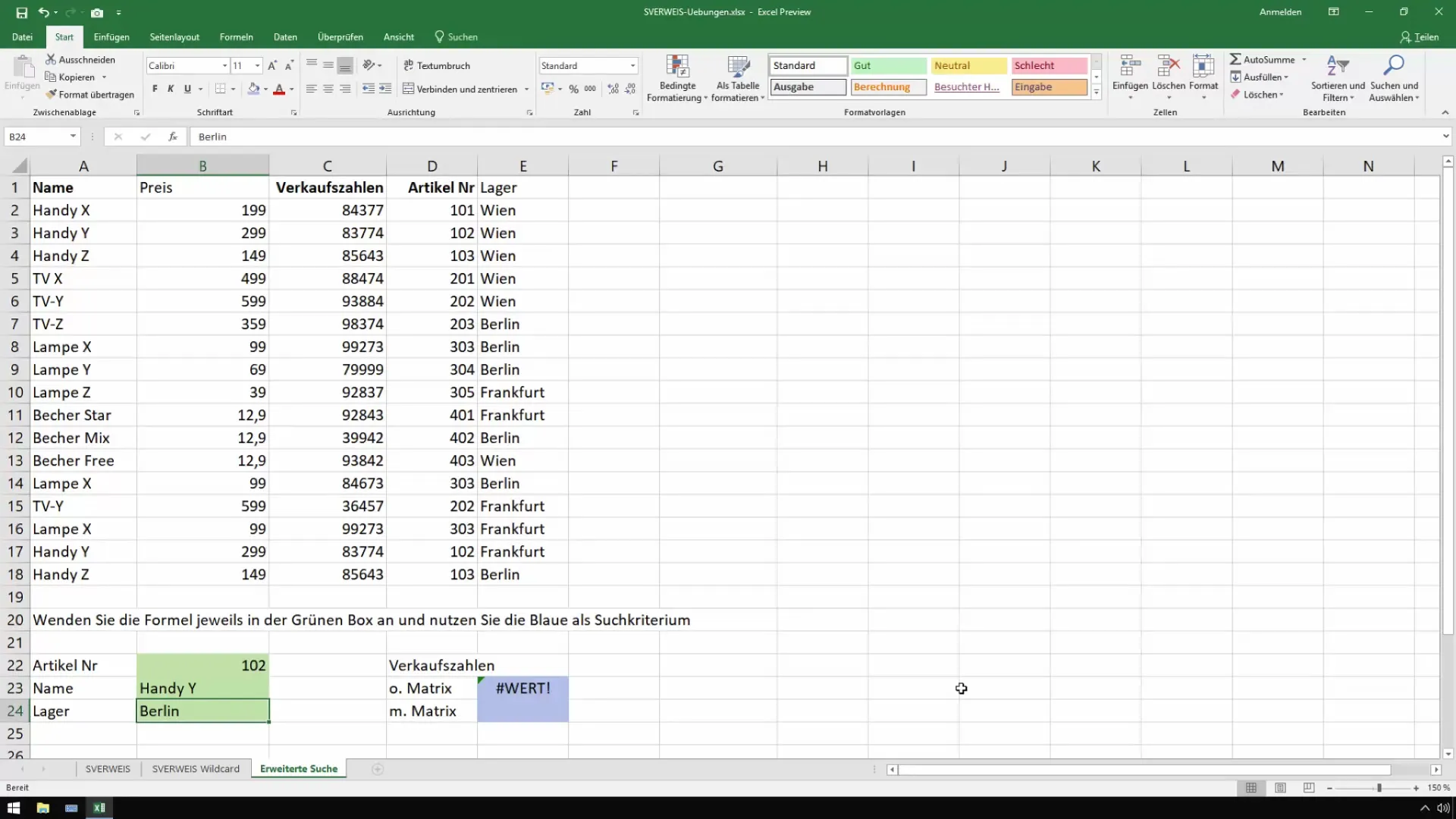
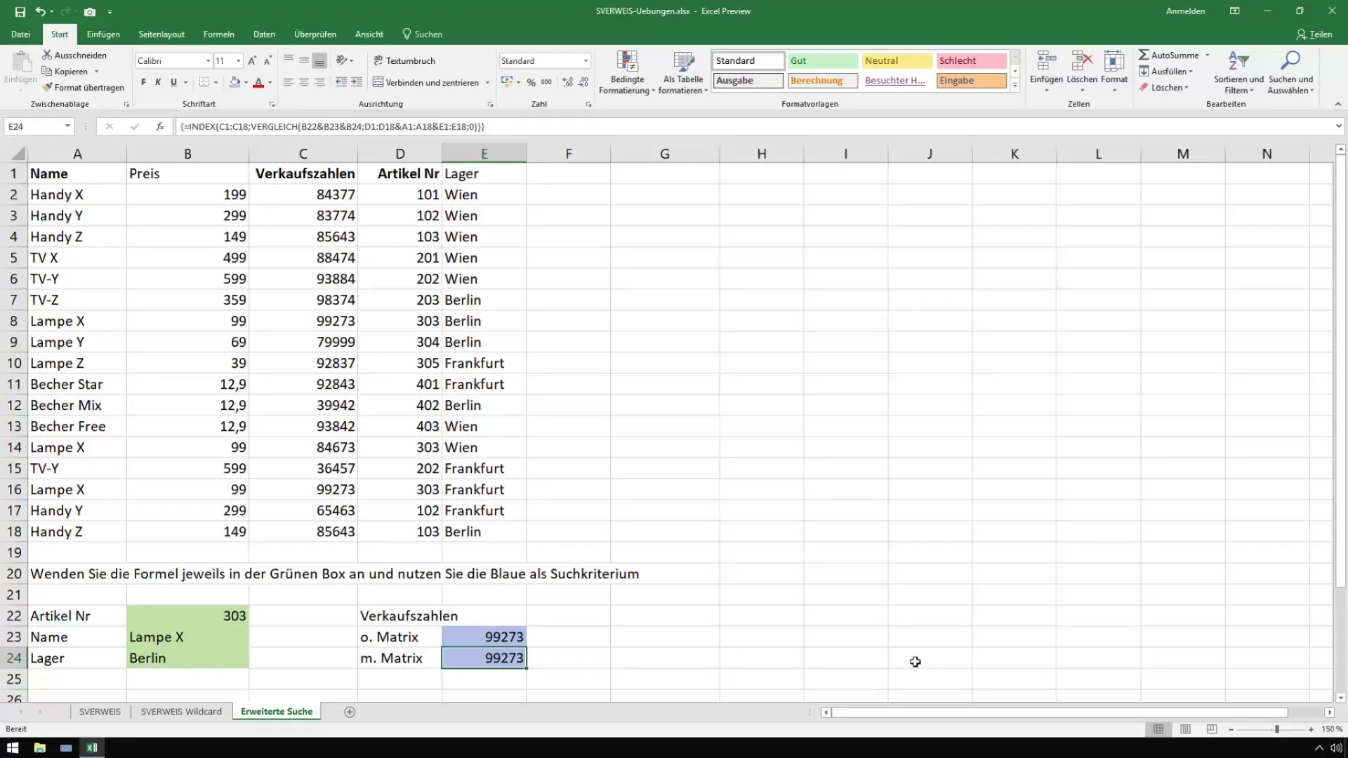
Step 10: Using Array Formulas

Another method to query the same data involves using array formulas. These ensure that your calculations are consolidated in one step and can improve clarity. Here, press Ctrl + Shift + Enter to activate the formula as an array function.

Step 11: Testing the Functions

Now test your created formulas with different inputs. For example, change the inventory storage and observe how the sales numbers adjust. This will help ensure that your formulas are functioning as desired.

Summary

Throughout this guide, you have learned how to use VLOOKUP across multiple columns to selectively query sales data and inventory levels. You have also discovered how to utilize more complex formulas using INDEX, SUMPRODUCT, and array formulas to optimize and simplify your data analysis.