Breaking down numbers into individual components with Excel

The effective manipulation of numbers and codes can be of great importance in the business world. Especially with long numbers such as credit card numbers or item numbers, it is often necessary to break them down into manageable and understandable parts. In this guide, I will show you how to work with the practical decomposition of numbers into parts in Excel. You will learn how to apply various functions to achieve a structured and clear representation.

Key Takeaways

• Number formats in Excel can be a challenge, especially when entering long digits.
• With Excel functions like LEFT, RIGHT, and MID, you can effectively break down numbers.
• Formatting is important to ensure that no data is lost.
• When dealing with sensitive data, it is crucial to take various security measures.

Step-by-Step Guide

Step 1: Enter numbers in text format

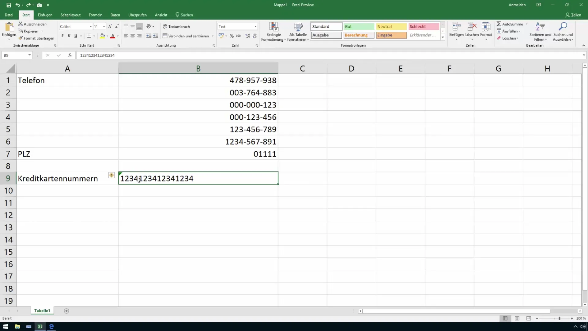
First, it is important to enter your credit card number or similar long numbers in text format. Go to Excel and make sure that the cell where you want to enter the number is set to text format. This prevents the number from being cut off in the default format.

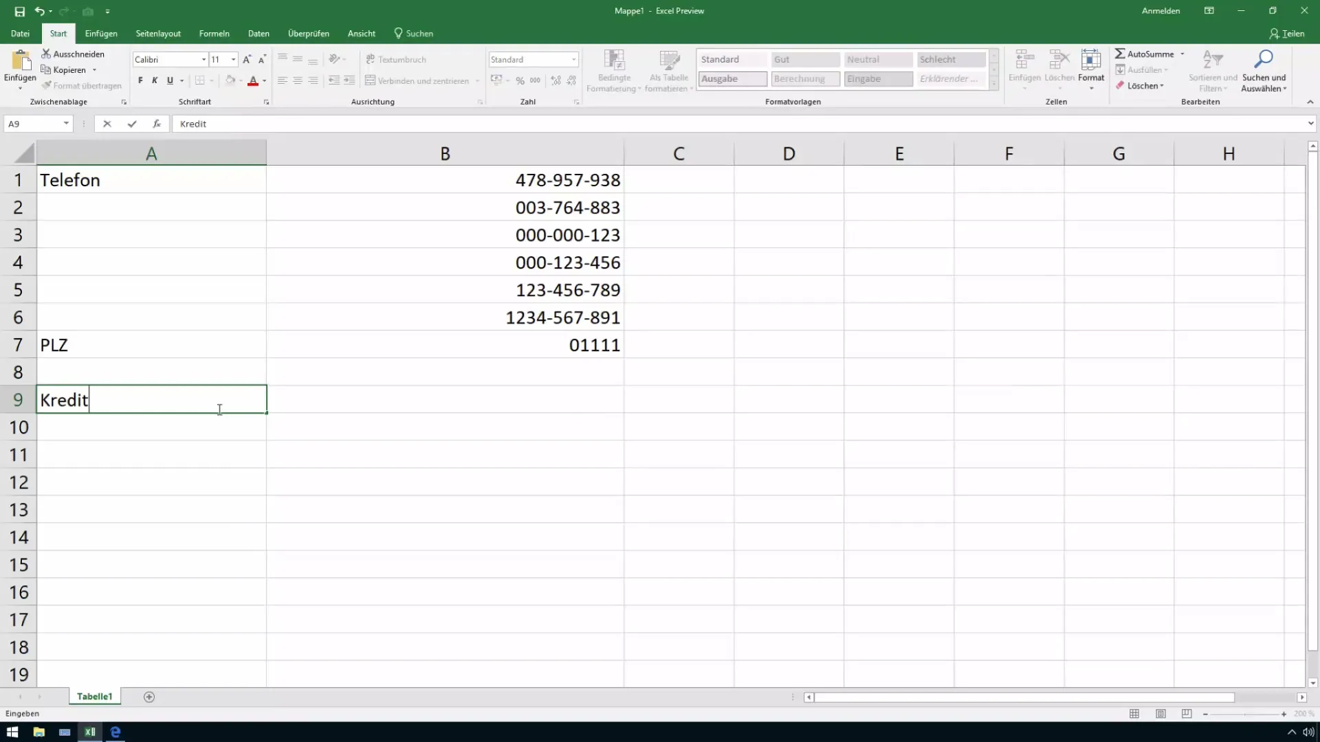
Once you have entered the numbers in text format, you can ensure that none of the last digits are lost. Make sure Excel shows the number as "saved as text" when you check it.

Step 2: Applying the "LEFT" function

To make the first four digits of your credit card number visible, use the LEFT function. In a new cell, input that you want to extract the first four characters from the cell with your credit card number. This looks like: =LEFT(A1, 4), where A1 is the cell with your credit card number.

The result shows you the first four digits of your number. This method is particularly useful to start structuring the number.

Step 3: Formatting numbers with a hyphen

To display the numbers more attractively, you can add a hyphen or space between the numbers. This is done by combining the functions together. Write: =LEFT(A1, 4) & "-" to add a hyphen after the first four numbers.

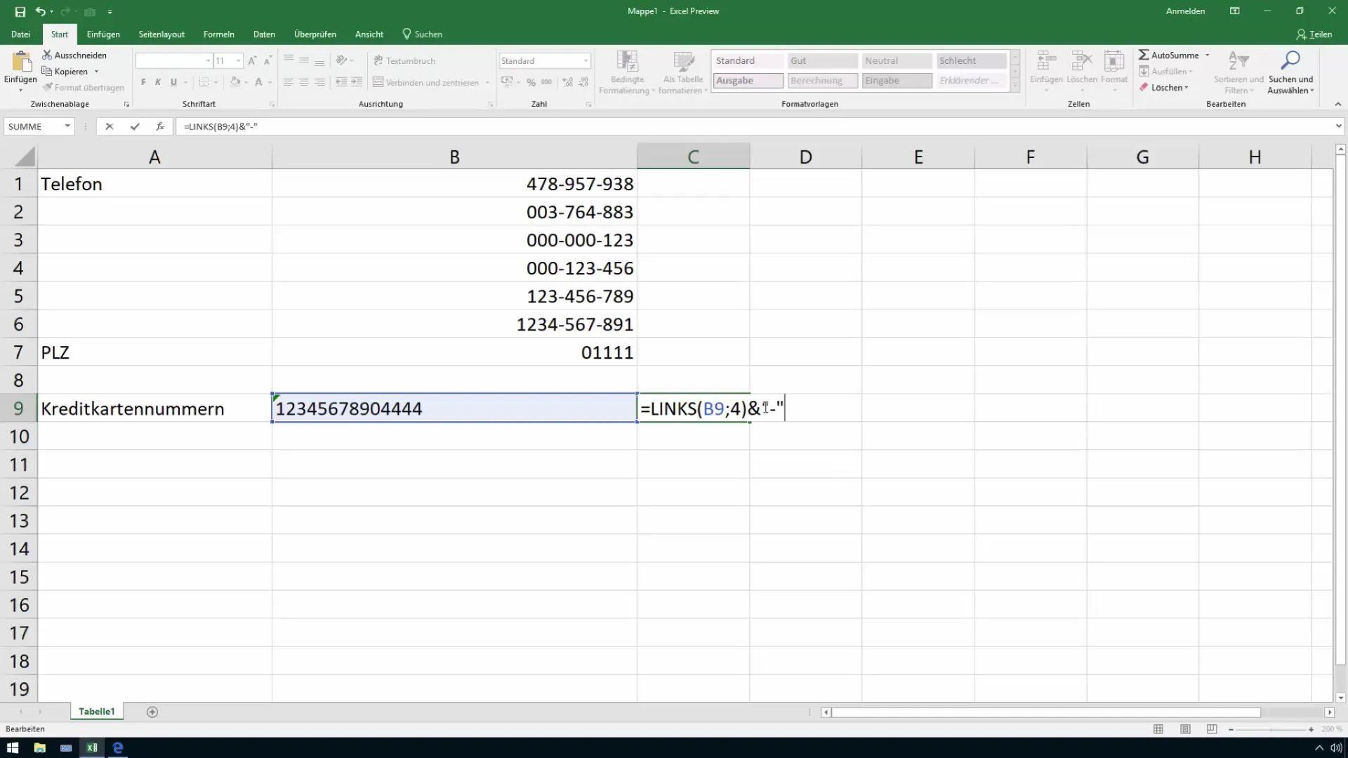
It already looks much better and makes the information more organized.

Step 4: Using the "MID" function

To extract the next block of numbers, you need the MID function. Suppose you want to have digits 5 to 8 from the credit card number, use the formula: =MID(A1, 5, 4).

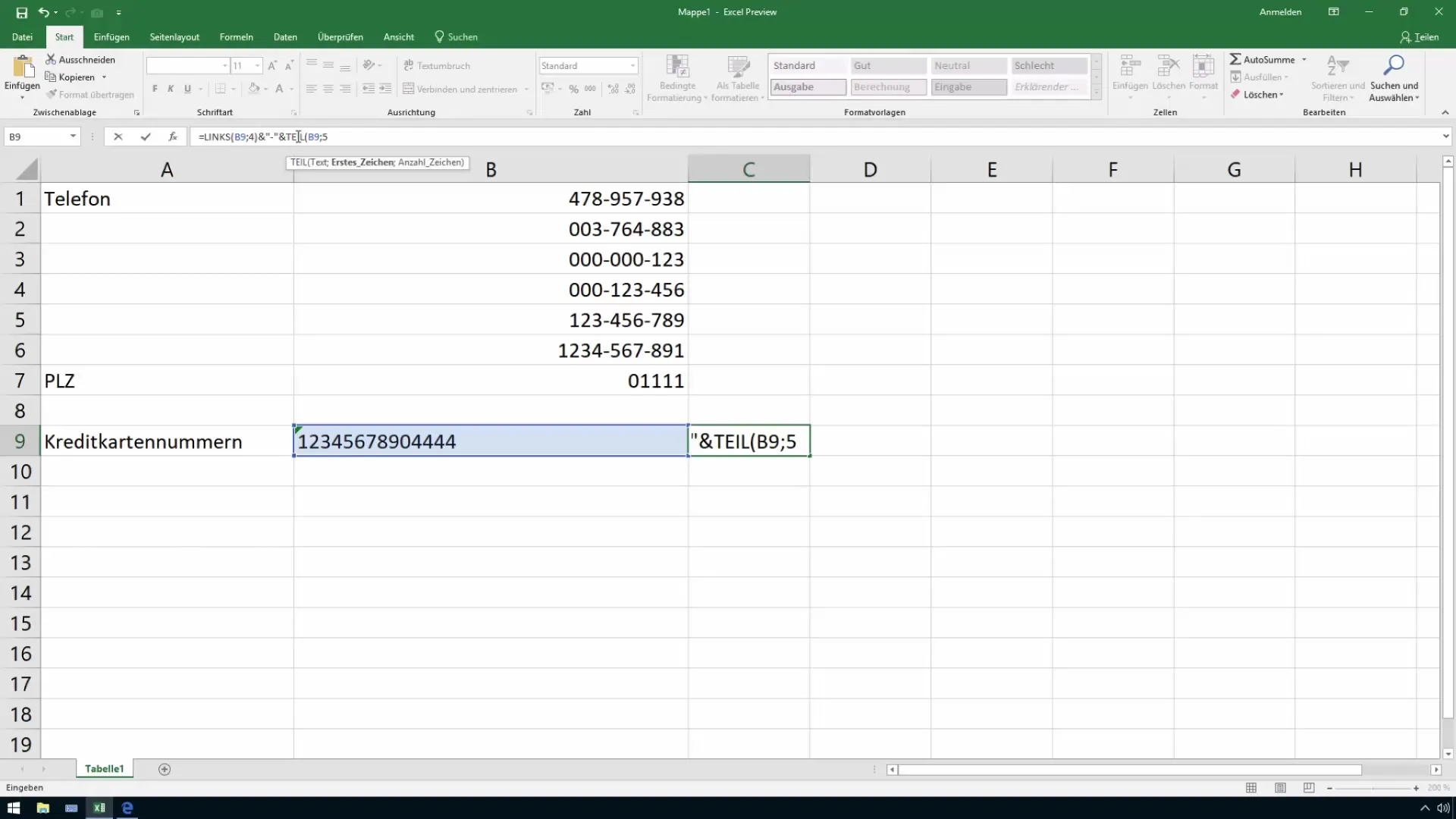
This formula starts at the fifth digit and returns four digits. Repeat this accordingly to get all blocks.

Step 5: Extracting the final digits with "RIGHT"

To get the last four digits of the credit card number, use the RIGHT function. It goes like this: =RIGHT(A1, 4).

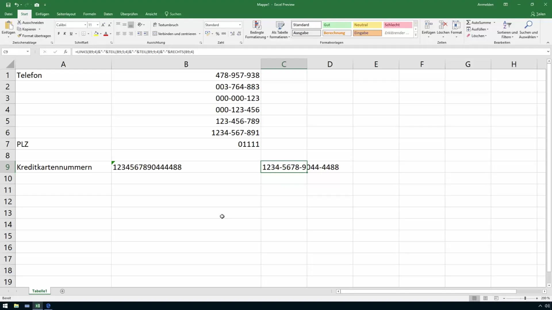
Now you also have the last group of digits and can format the entire credit card number in the desired format.

Step 6: Final formatting and data checking

After extracting all parts, combine everything in one cell. An example could look like this: =LEFT(A1, 4) & "-" & MID(A1, 5, 4) & "-" & RIGHT(A1, 4).

Remember to be very careful when using credit card data. Data should be anonymized and handled securely.

Step 7: Take security measures

Finally, it is important to also consider the security of the entered information. Sensitive data must be protected accordingly to comply with data protection regulations.

You can set up encryption or password protection for your Excel file to protect the data.

Summary

You have now learned how to effectively break down long numbers in Excel. You can use various functions to create formats and structures that help you present the information clearly. Pay attention to the sensitivity of the data you are working with and implement appropriate security measures in your work.