Determine sales ranks efficiently - an Excel guide

Discover how you can effectively analyze sales ranks in Excel to identify your top sellers and slow-moving products. In this guide, I will explain to you step by step how to evaluate sales figures without having to manually sort your list. With the right functions, you can easily and quickly generate the desired results and maintain a clear overview of your products.

Main Insights

• Using the MIN and MAX functions allows you to quickly determine the best and worst sales values.
• Utilizing the RANK, LARGE, and SMALL functions enables a precise analysis of sales ranks.
• The VLOOKUP is crucial for linking product-related information with sales figures.

Step-by-Step Guide

Insert Sales Figures into an Excel Document

First, you need a table with sales figures. Create a new file in Excel and name it "SalesRank.xlsx". Enter your sales figures and corresponding products in the columns, so you have a clear representation. In our example, you have products like cell phone, TV, and lamp along with their sales figures.

Applying MAX and MIN Functions

To automatically determine the best and worst rankings, we will use the MAX and MIN functions. First, name your sales figures so that you can work easier in the formulas. For example, you can define the range of your sales figures as "SalesNumbers".

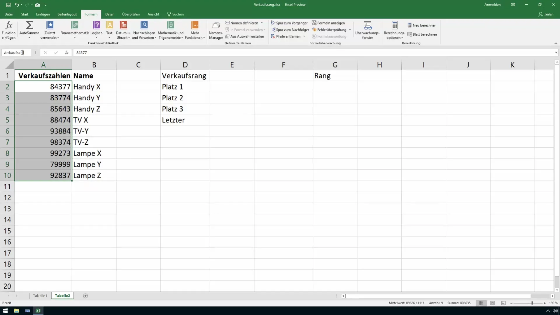
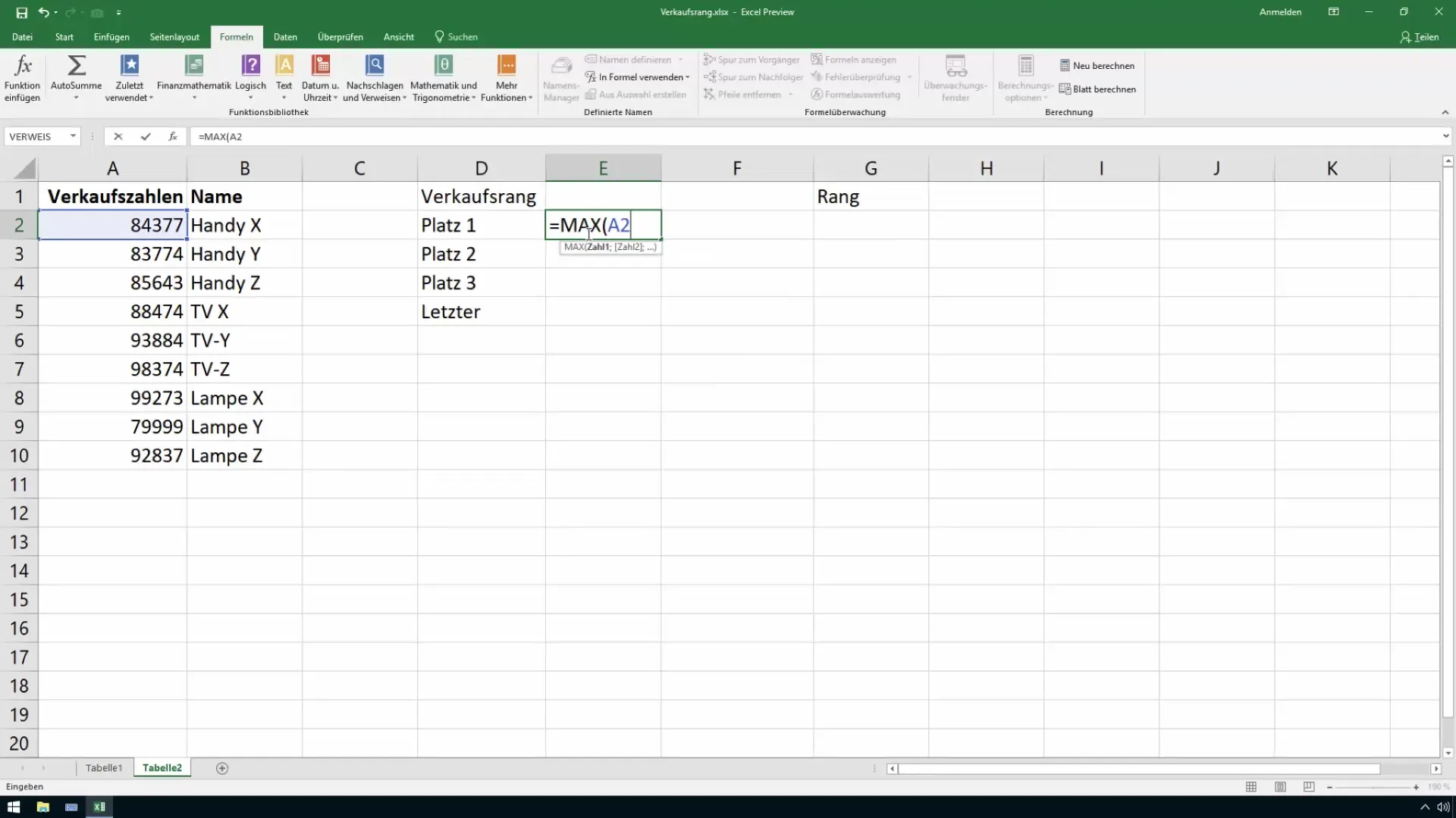
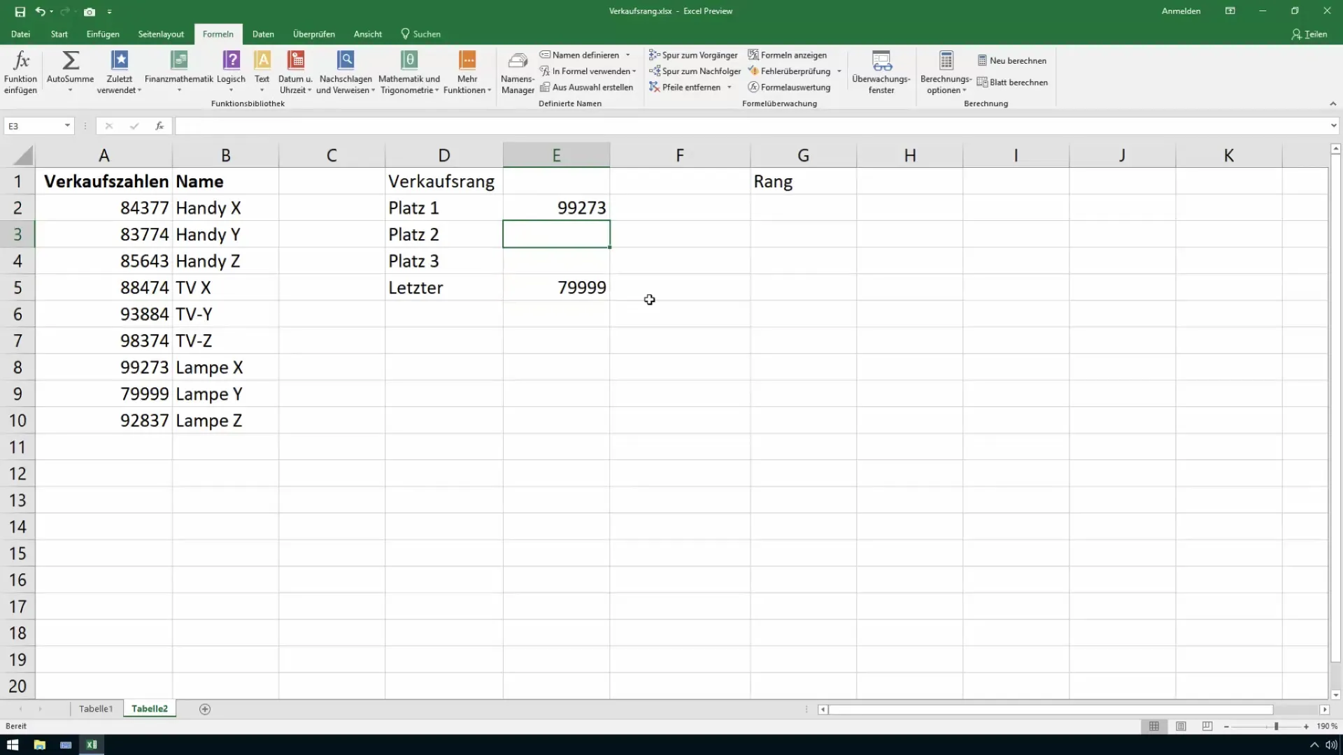
Now you can use the formula "=MAX(SalesNumbers)" in a cell. This will display the highest sales value, which is the 1st place.

For the lowest sales value, write "=MIN(SalesNumbers)". Now you can easily see which number is the lowest and thus holds the 9th place.

Determining Ranks with LARGE and SMALL

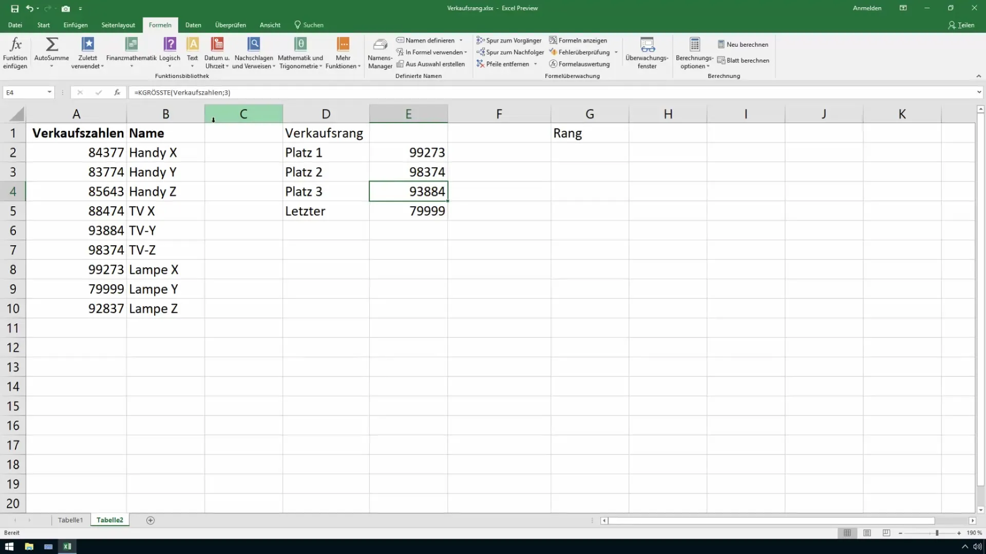
Using the LARGE function, you can determine not only the best sales value but also the second and third place. Simply enter "=LARGE(SalesNumbers;2)" for the second place and "=LARGE(SalesNumbers;3)" for the third place. The same applies to the SMALL function to determine the worst sales numbers.

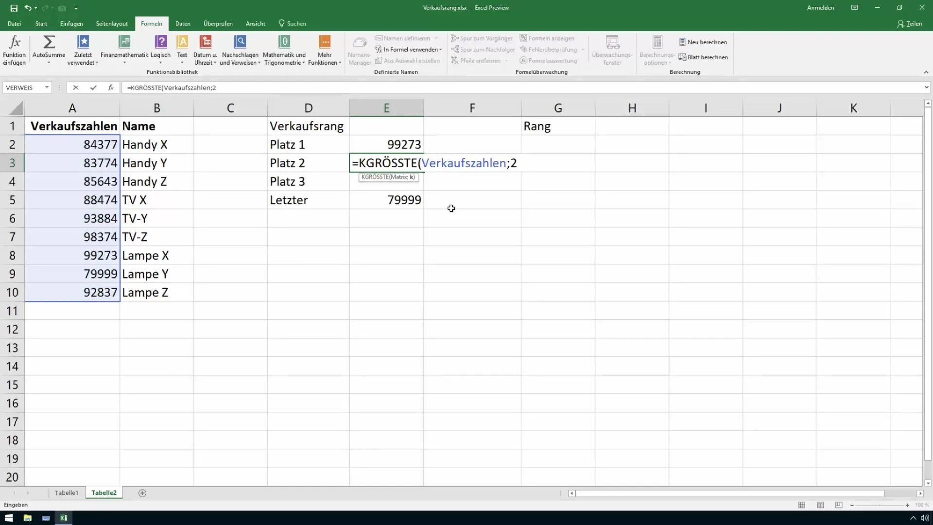
When you drag these formulas down, you can quickly list all ranks in a column.

Assigning Products to the Ranks

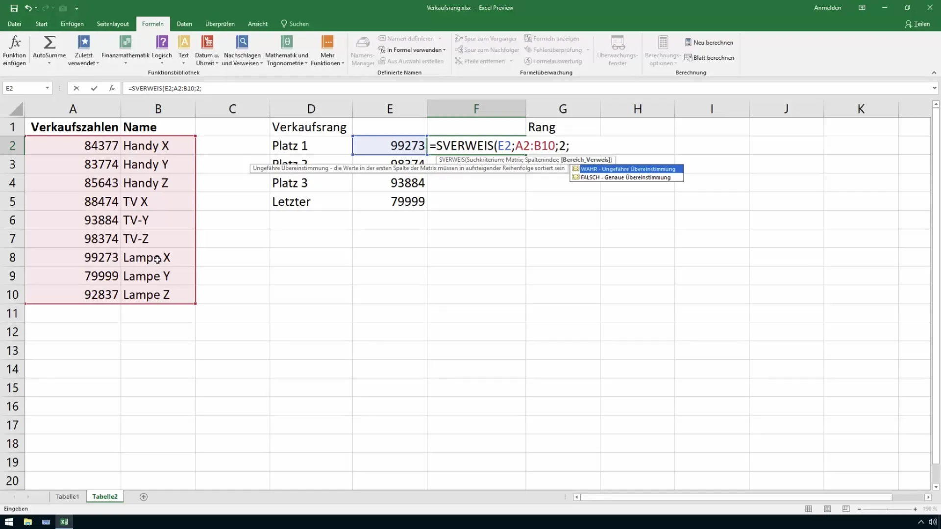
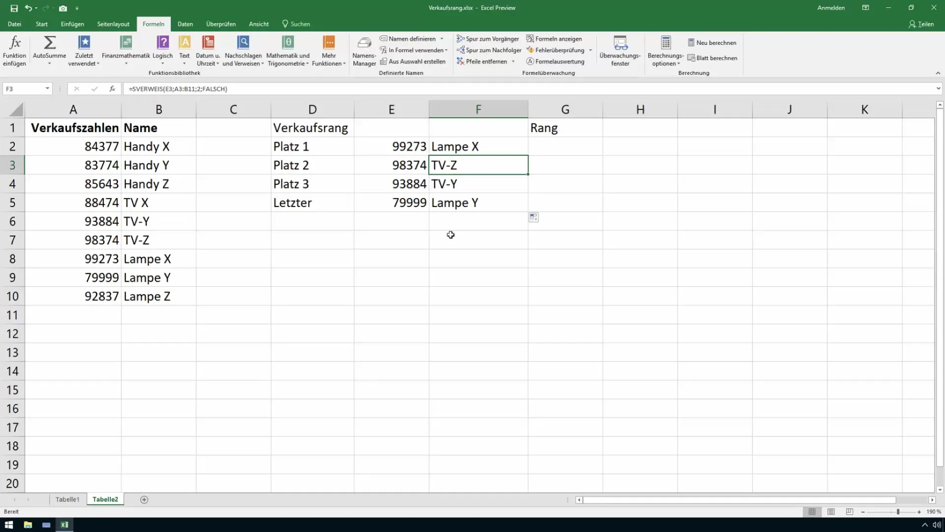
To assign the products to the determined ranks, you perform a VLOOKUP. The syntax looks like this: "=VLOOKUP(MAX(SalesNumbers);A2:B10;2;FALSE)". Here, you search for the highest sales number in your lookup array, which is composed of the sales figures and the corresponding product names.

Drag the VLOOKUP down to see the product names for all entered sales values.

Sort the Ranks

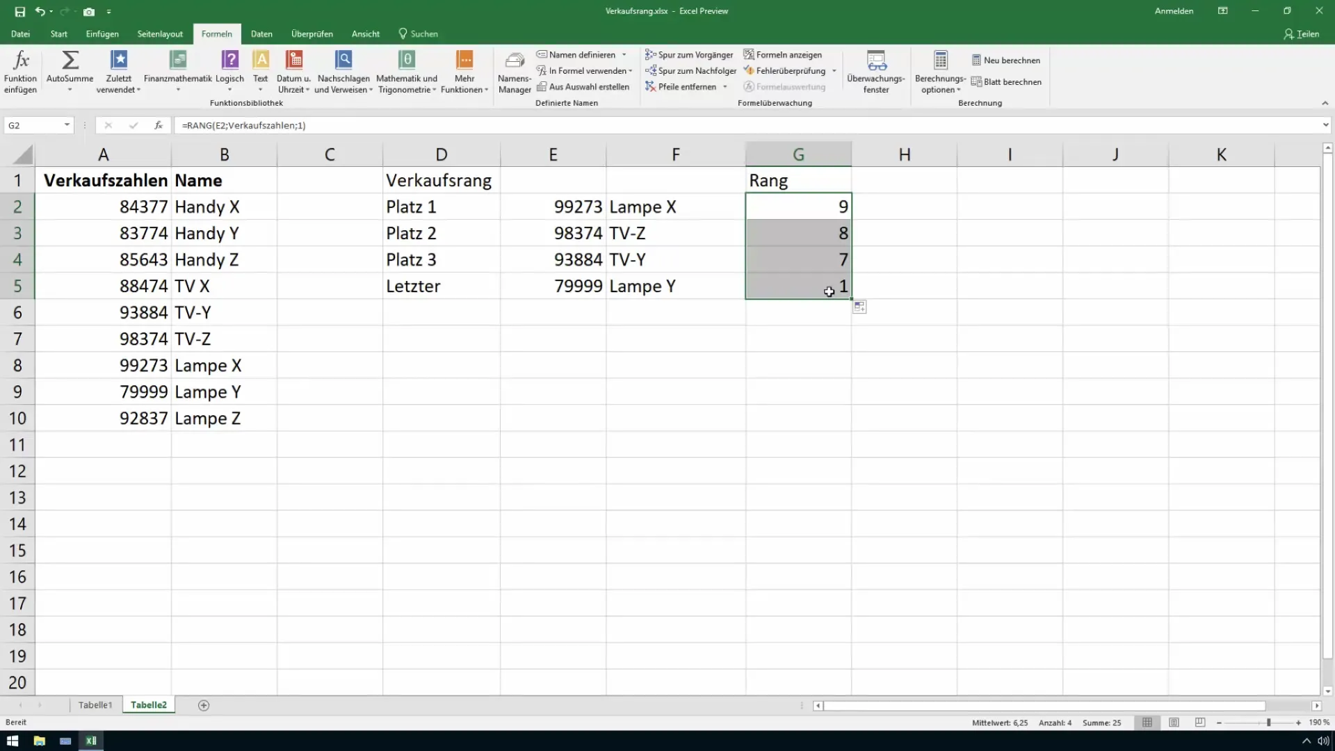
Another way to present sales figures clearly is rank sorting. Use the function "=RANK(Number;SalesNumbers;0)" to determine the ranking order of the sales numbers. Set the third argument option to 0 to sort the order from highest to lowest value.

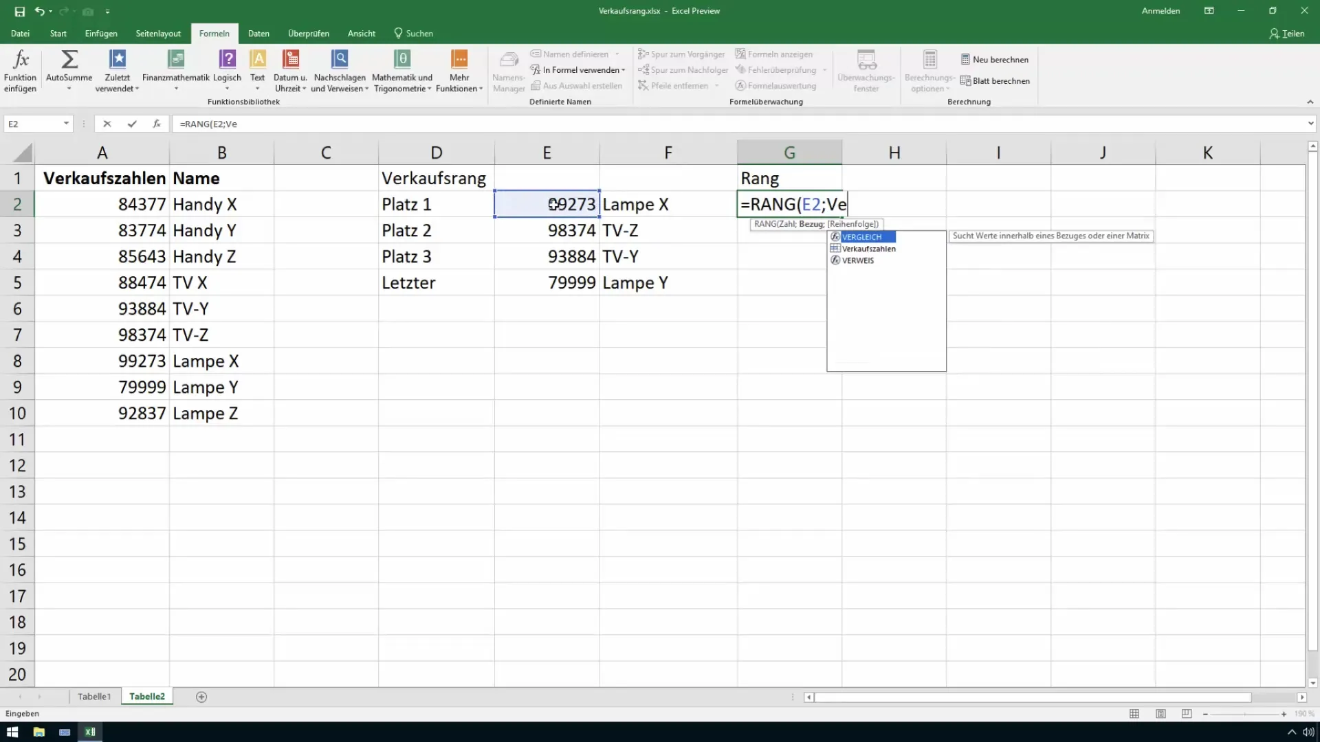
If you want to sort the ranks in ascending order, change the last argument to 1. Now you can see which products have the lowest sales numbers.

Summary

In this tutorial, you have learned how to automatically evaluate and sort sales figures with Excel. Functions like MAX, MIN, LARGE, SMALL, and VLOOKUP quickly give you an overview of your top sellers and slow movers. Use these techniques to analyze your sales data more effectively and make informed decisions.