If you are looking for a simple and effective method to highlight late delivery dates in Excel in controlling or sales, you have come to the right place. In this tutorial, you will learn how to use conditional formatting to make your data visually appealing and easy to understand. You will learn to identify and visually represent the differences between planned and actual delivery dates. This will not only help you analyze your orders, but also identify potential issues early on.
Main Takeaways
- Conditional formatting allows you to highlight delivery dates with colors.
- With simple formulas, you can determine whether deliveries are on time.
- You will learn how to customize conditional formatting rules to accommodate varying deadlines.
Step-by-Step Guide
Step 1: Prepare Your Data
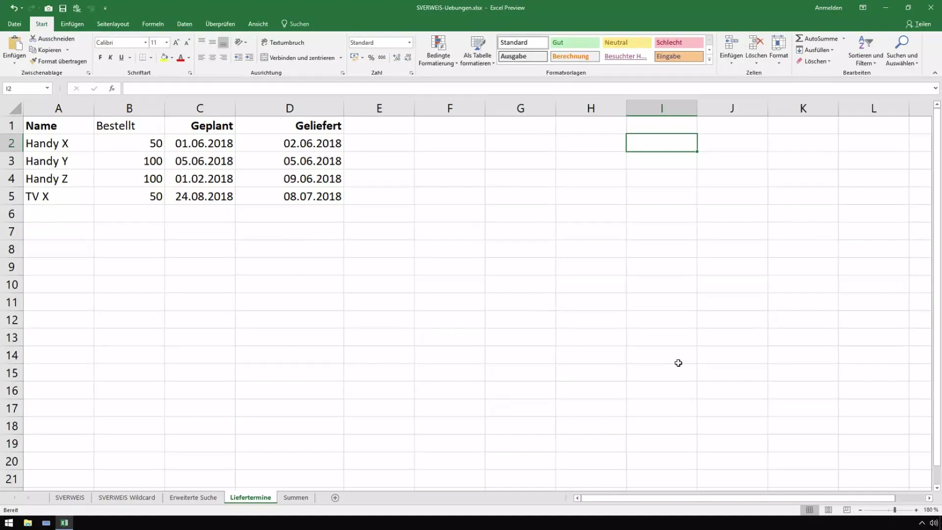
First, it is important to prepare your data in Excel. Create a table with your orders, including at least the columns for the planned delivery date and the actual delivery date. Make sure the data is properly formatted so that Excel can interpret it correctly.
Step 2: Select Cell Range
After entering your data in Excel, select the cell range you want to format. Make sure not to include the headers as you only want to analyze the relevant data.
Step 3: Apply Conditional Formatting
Go to the "Conditional Formatting" menu in the Excel interface and choose "New Rule". Here, you can create a rule that specifies the criteria for highlighting the cells.
Step 4: Create Rule for Late Deliveries
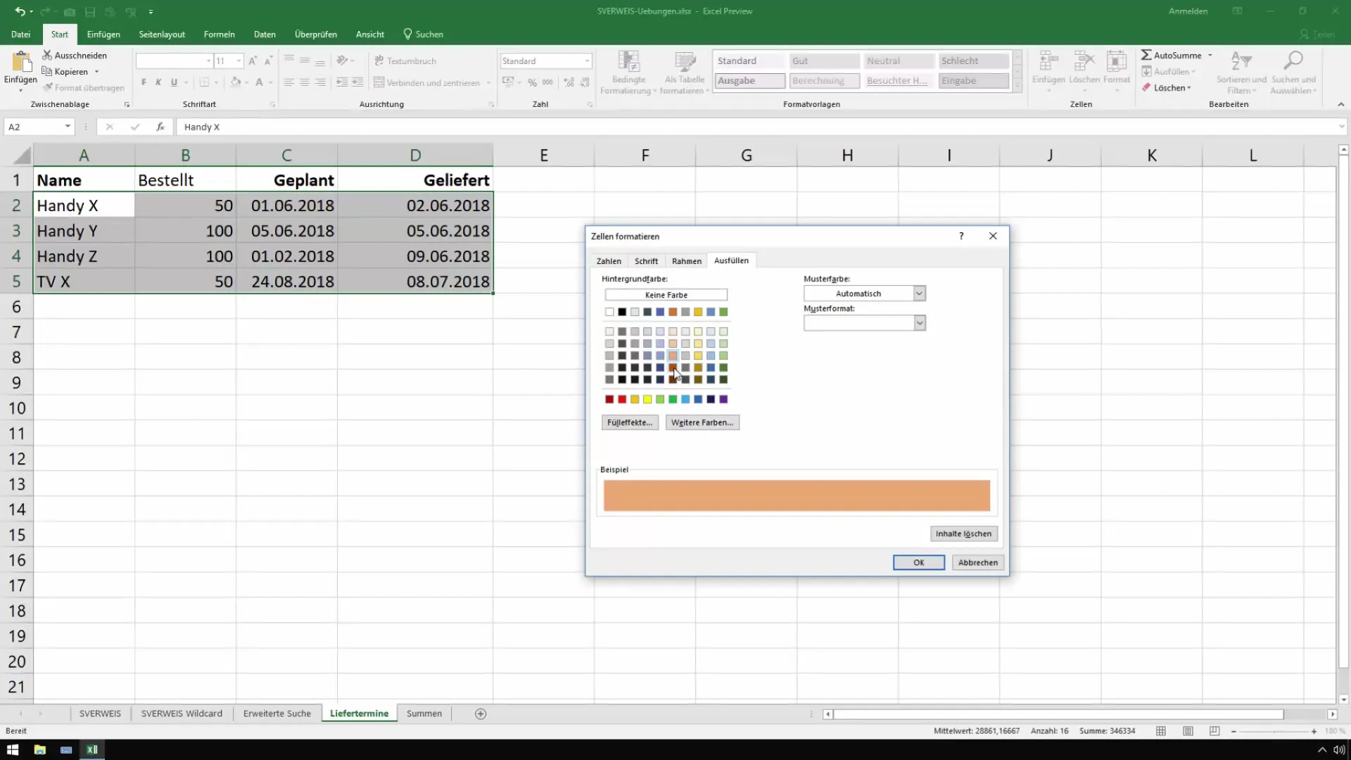
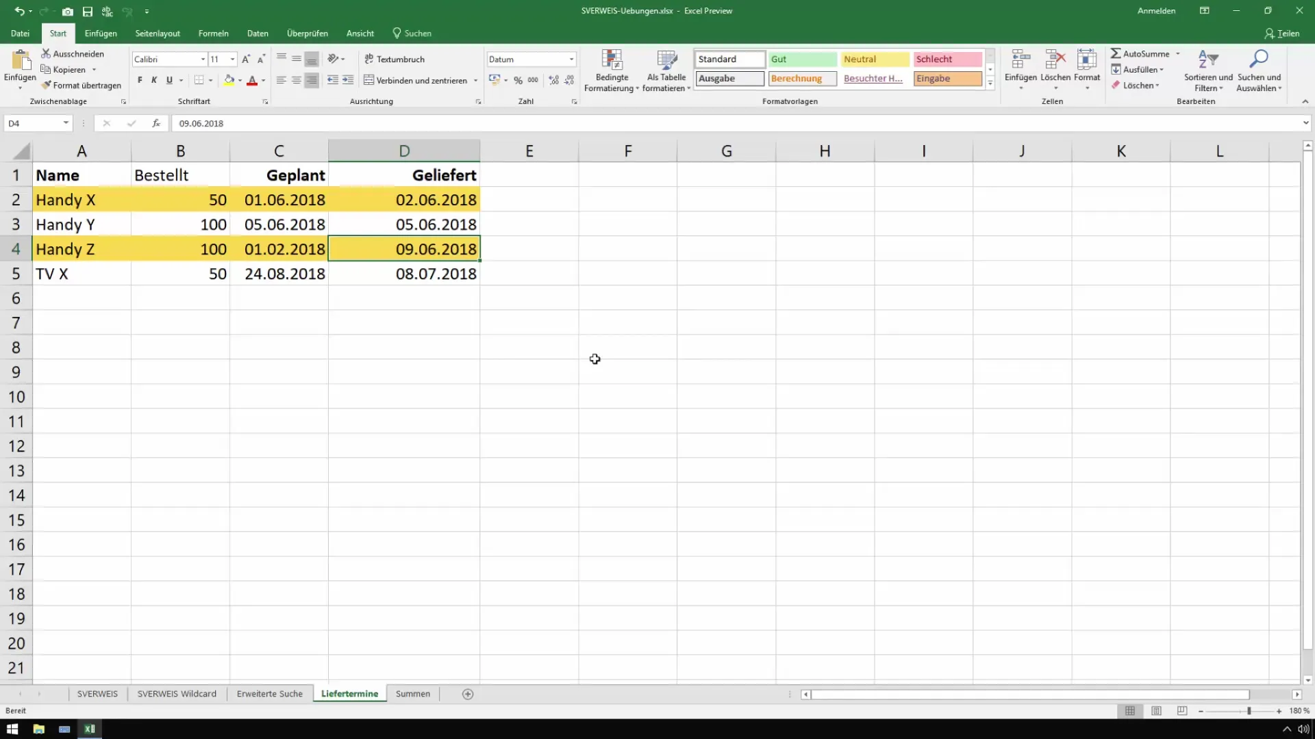
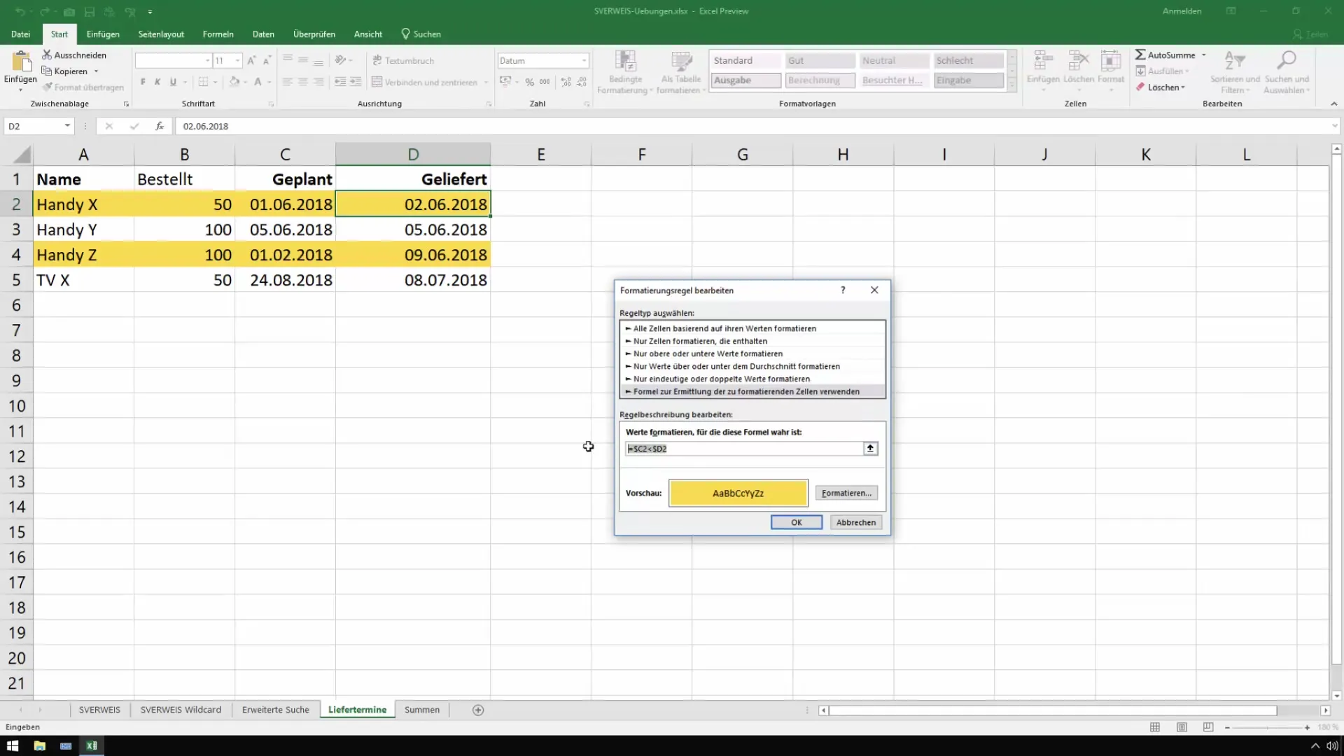
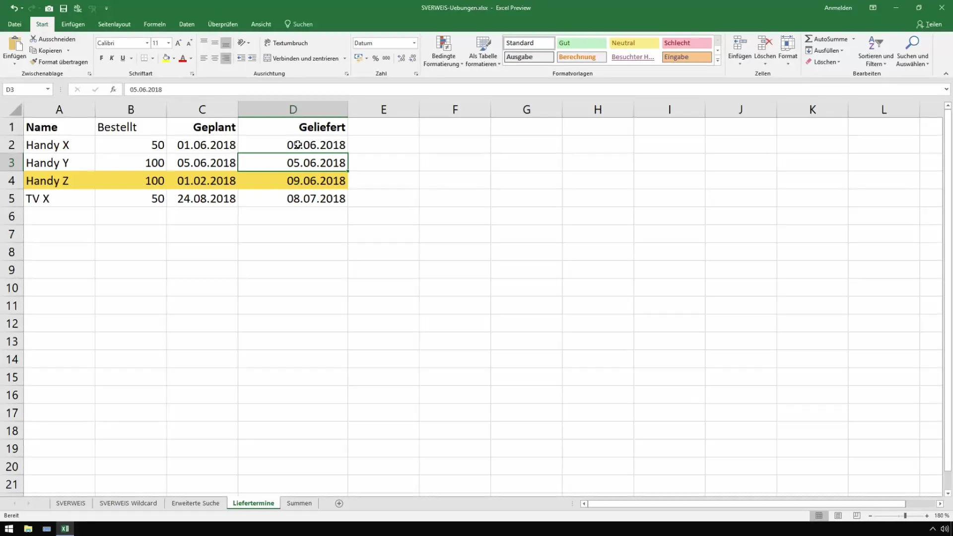
To create the rule, use a simple formula. You want Excel to check if the planned delivery date is less than the actual delivery date. Use referencing for the columns, for example, for the planned date as $C2 and for the actual date as $D2. The formula would look like this: =C2 Now it's time to define the appearance of the highlighted cells. Choose a striking color, such as a vibrant orange, to clearly indicate delays. Confirm your selection with "OK". After applying the rule, you will now see that Excel has highlighted the late deliveries with colors. For example, an order scheduled for February but delivered in June would be clearly visible. This allows you to quickly identify where issues occurred. To create more flexible rules, you can adjust the previous rule. For example, you can specify that a delivery date is acceptable even if it is up to three days after the planned date. You can edit the existing rule through the "Manage Rules" menu. Now, you need to slightly modify the formula. Instead of just checking if the planned date is less than the actual date, subtract the planned date from the actual date and check if the difference is greater than two days. The new formula could look like this: =(D2-C2)>2. Once you have changed the formula, review the results again. Delays of over three days should now be correctly highlighted, while all deliveries with less than three days of delay will retain their original status. Highlighting late delivery dates in Excel can be done quickly and easily with conditional formatting. By understanding the formulas and applying the formatting options correctly, you can make your data much more organized. This way, you can keep track of your deliveries and react in a timely manner if necessary. How can I remove the conditional formatting?You can manage and remove the rule using the "Conditional Formatting" menu. Can I change the color of the highlight?Yes, you can adjust the color in the formatting options at any time. What happens if the data is not formatted correctly?Excel may not recognize the data correctly, leading to inaccurate results. Do I need special Excel skills for this guide?No, the steps are simple and understandable even for beginners.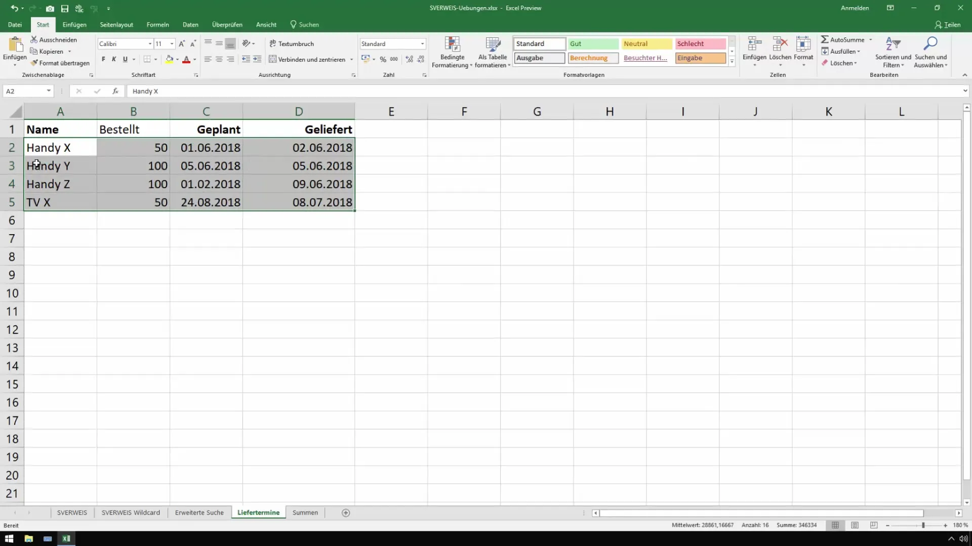
Step 5: Select Formatting Options
Step 6: Review the Results
Step 7: Adjust the Rule for More Flexibility
Step 8: Modify the Formula
Step 9: Review the Adjusted Results
Summary
Frequently Asked Questions

