Create colored gridlines in Excel

Excel offers numerous ways to visualize data, and one often overlooked feature is the gridlines. Navigating through extensive datasets can be a challenge. Especially when having multiple worksheets in one file, it is helpful to add colorful accents. This way, you not only keep an overview but also ensure that you are always working in the correct worksheet. In this guide, you will learn how to set up and use colorful gridlines in Excel to make your work more efficient.

Main Takeaways

You can replace the default gray gridlines in Excel with colorful line settings to make your workbooks visually appealing and simplify the differentiation between different worksheets. This way, you keep track and work more effectively.

Step-by-Step Guide

1. Open Excel File

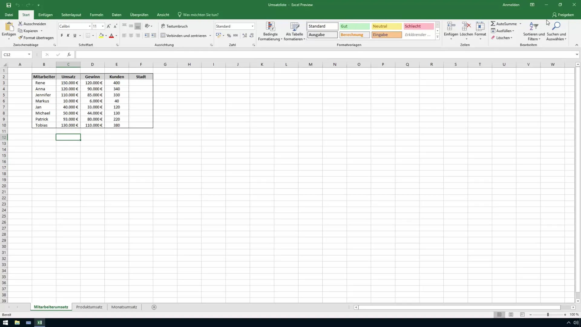
First, open the Excel file in which you want to adjust the gridlines. In our example, we are working with a file named "Sales List". This file shows you the basic structure of the data you want to work on.

2. Select the Right View

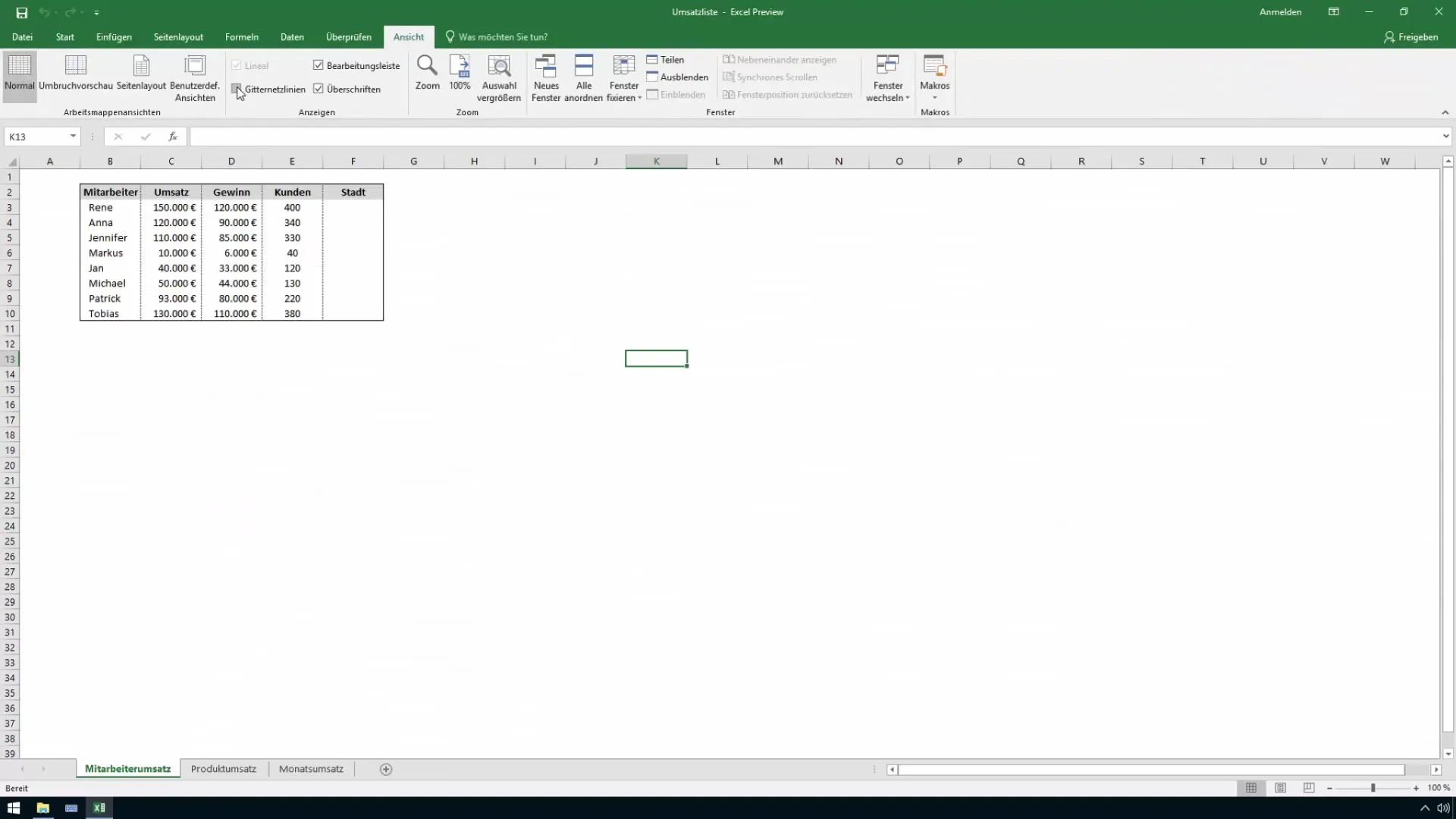
Once you have opened the file, you will notice that the default gridlines are gray. Sometimes, these can make data in large tables harder to read. However, you can also hide them to get a clearer view. To do this, go to the "View" tab and select the option that allows you to hide the gridlines.

3. Access Options

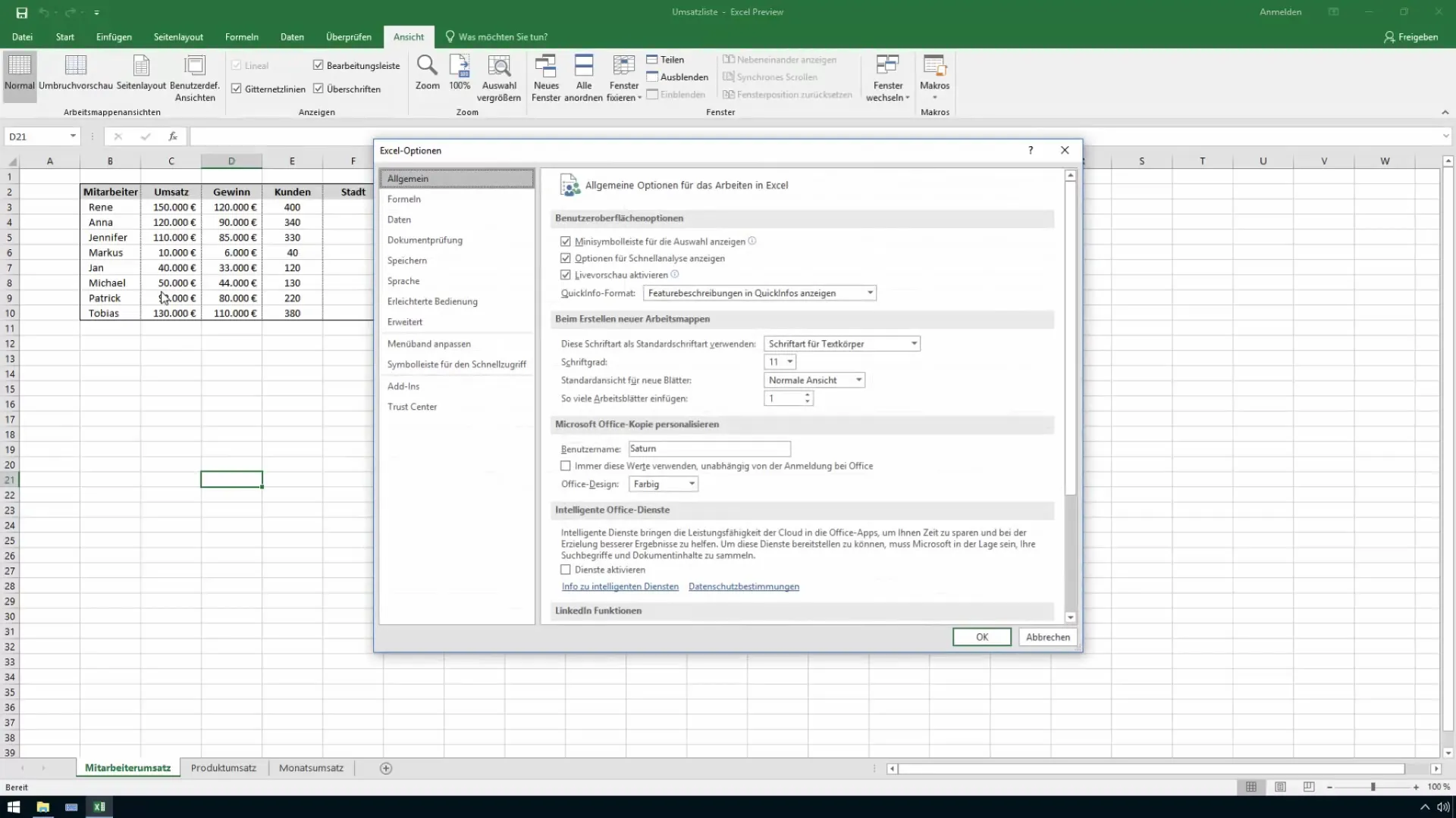
To enable colorful gridlines, you need to access Excel's options. You can do this by clicking on "File" and then selecting "Options". A new window will open where you can customize various settings.

4. Find Advanced Settings

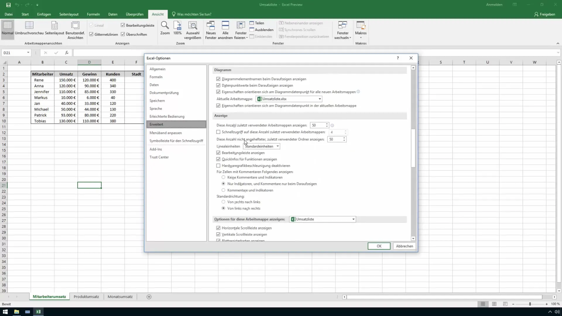
In the options menu that opens, scroll down until you find the "Advanced" section. Here you will find numerous customization options, including setting the gridlines.

5. Color the Gridlines

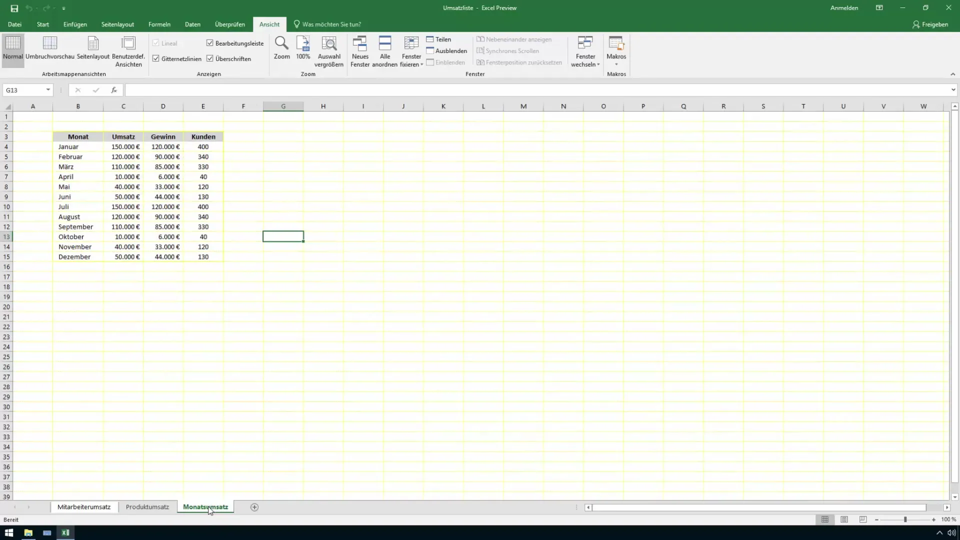
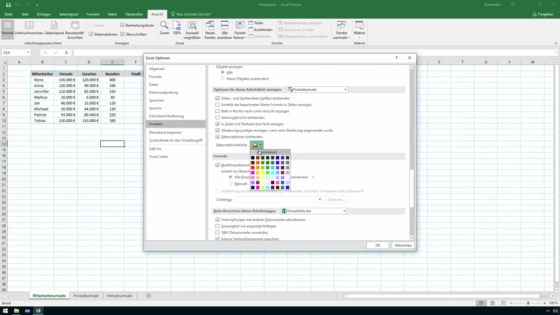
In the advanced options, you will find the point where you can adjust the gridlines for selected worksheets. Choose the appropriate options there to set different line types for the employee, product, and monthly sales sheets. For example, you could use light blue lines for employee sales data and reddish lines for product sales.

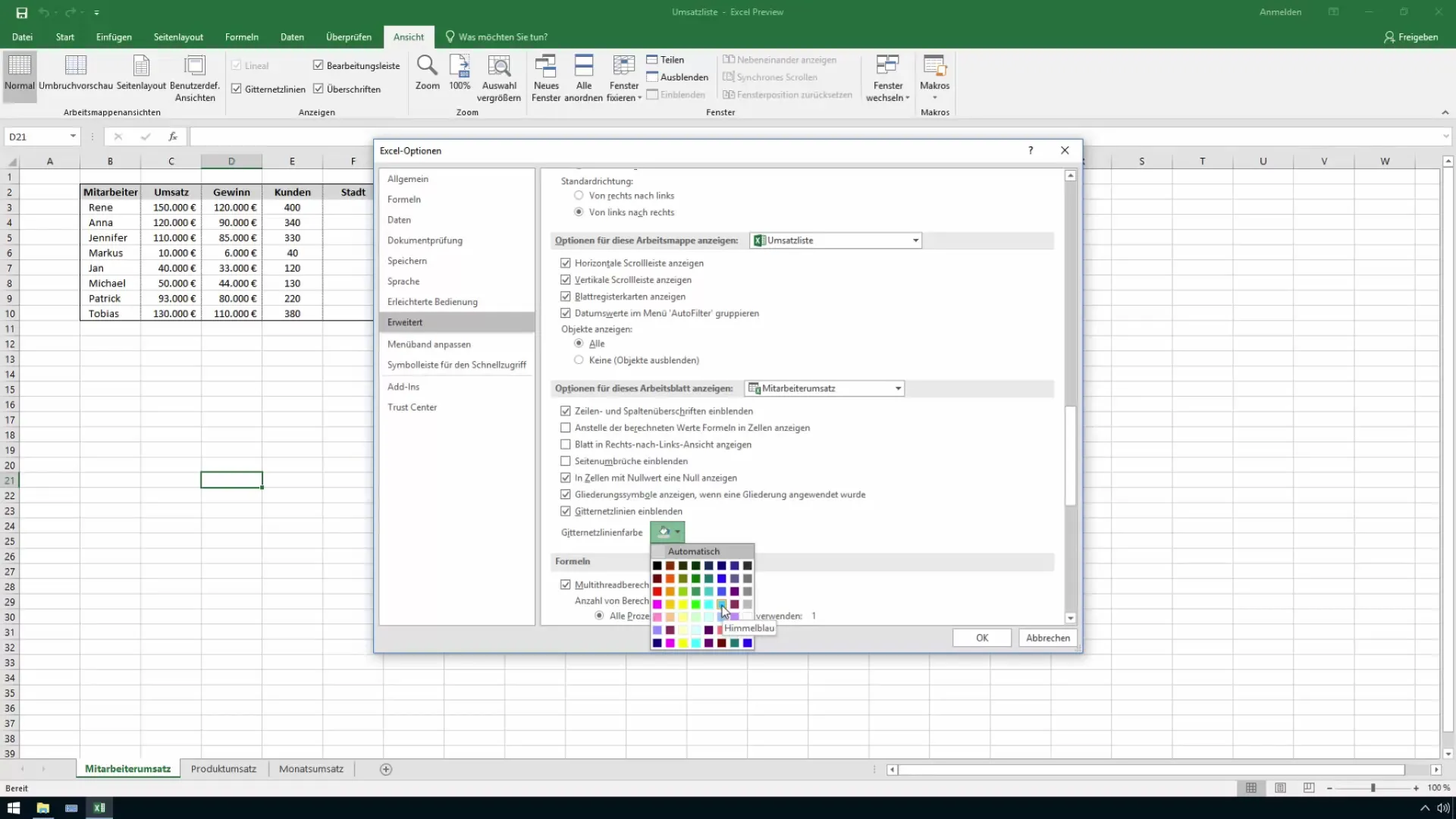
6. Choose Colors and Confirm

Select the desired colors and click "OK" to save your changes. If done correctly, you will see the colorful gridlines in your Excel table, significantly enhancing the data structure.

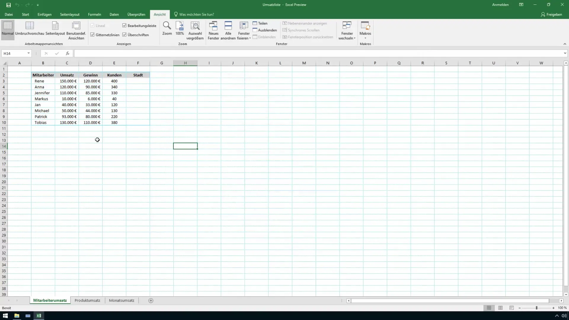
7. Monitor Adjustments

Now you can better secure the table and make color adjustments as needed. Experiment with different colors to find out which combinations help you best differentiate between the various worksheets.

8. Undo Changes

If you are not satisfied with the changes, you can always undo them. Simply go back to the options, select the "Advanced" section, and reset the colors to the default values.

Summary

Adjusting the gridlines in Excel can make a significant difference in user experience by improving clarity and differentiation between different data sets. Experiment with different colors to make your Excel workbooks more personal and functional.