Transpose columns and rows in Excel

With Microsoft Excel, you can not only save and analyze data, but also easily adjust your table structure. Sometimes you have a well-structured table, but the arrangement of columns and rows does not fit your needs. This is where the Transpose function comes into play – a quick and practical way to switch data from horizontal to vertical and vice versa without having to manually change everything afterwards. This guide gives you a step-by-step overview of how you can effectively use the Transpose function to improve the clarity of your data.

Main Insights

• The Transpose function allows you to flip columns and rows of a table.
• You can simply copy data and paste it transposed at the desired location.
• With just a few clicks, you can achieve an attractive and handy data structure that facilitates your work.

Step-by-Step Guide

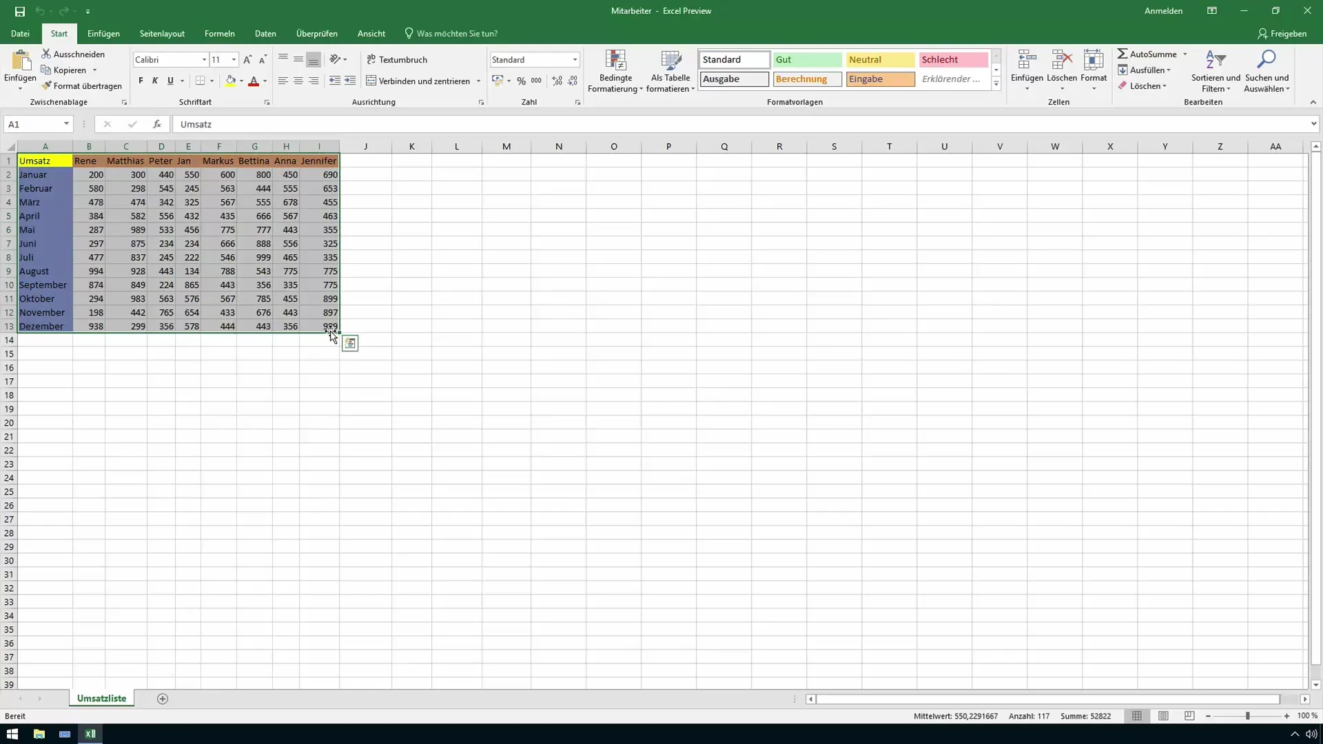
First, take a look at the table you want to transpose. For example, you have an employee table sorted by revenue and employees. It may be that the arrangement does not meet your expectations, and you would prefer to present the data with employees listed vertically and months listed as columns.

To start, select the range of the table you want to transpose. In this example, it's the revenue table for employees from Rene to Jennifer. So, you mark this range that you want to reverse.

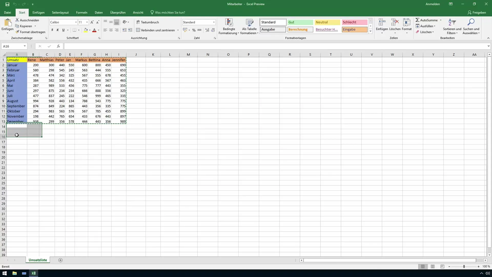
Now it's time to copy the data. To do this, click on the "Copy" button under the "Home" menu. This step is necessary to paste the data later back at the desired location, albeit in a reversed form.

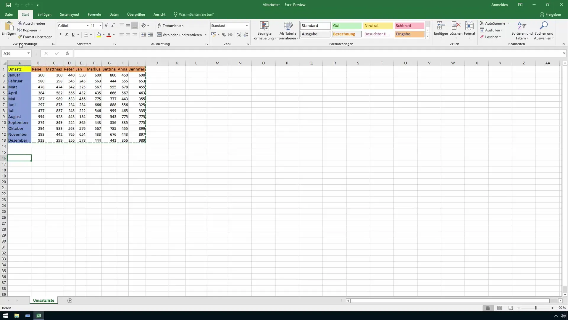
After copying, select the new range where the transposed data is to be pasted. Remember that the rows shift in width, so choose enough space.

Now comes the crucial step: Click on "Paste" and then on the small arrow to see more paste options. Here you will find the special field that allows you to transpose the data.

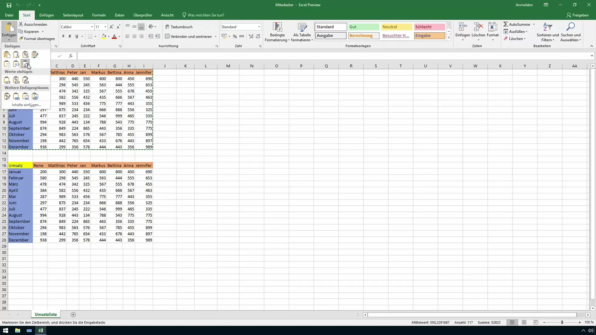
Once you click on the Transpose option, you will immediately see a preview of the transposed table. Now it's clear: the data is displayed exactly in reverse. Employee Markus now has his 600 in January and his 563 in February, and the overview is significantly improved.

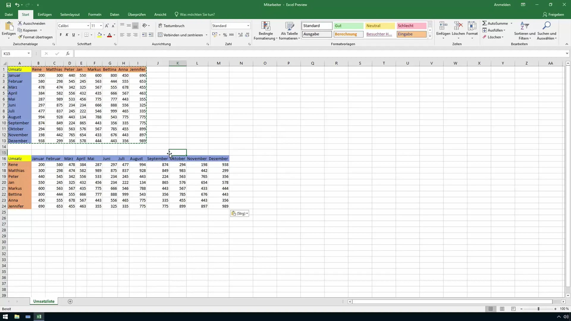
With a simple click, you have changed the arrangement of the table, and that without complicated formulas or formatting. It's so simple that you can also use this function for other employee tables or any other data structure.

This short lesson shows that the Transpose function not only saves time but also significantly improves the structure of your data. Sometimes it's the small tools that have the greatest impact on your efficiency in the office. Consider where you can apply this technique in your daily work or in other Excel documents.

Summary

The Transpose function in Excel is a simple yet powerful tool that allows you to quickly and effectively change the arrangement of data. By copying and pasting, you can improve the clarity of your tables and save time. With this guide, you will learn how to make optimal use of the Transpose function.