Hide rows and columns in Excel

Working with Excel can sometimes be challenging, especially when dealing with large tables with a lot of data. In this guide, I will show you how to efficiently hide rows and columns in a table to get a better overview. Hiding unnecessary information can increase your working speed and allow you to focus on the truly important data.

Main Insights

• You can easily hide columns and rows in Excel.
• Unhiding hidden layers is also intuitive.
• By selectively hiding, you increase the clarity of your tables.

Step-by-Step Guide

To illustrate hiding rows and columns in Excel, we will use a movie list as an example. Follow these steps to make the most of your data.

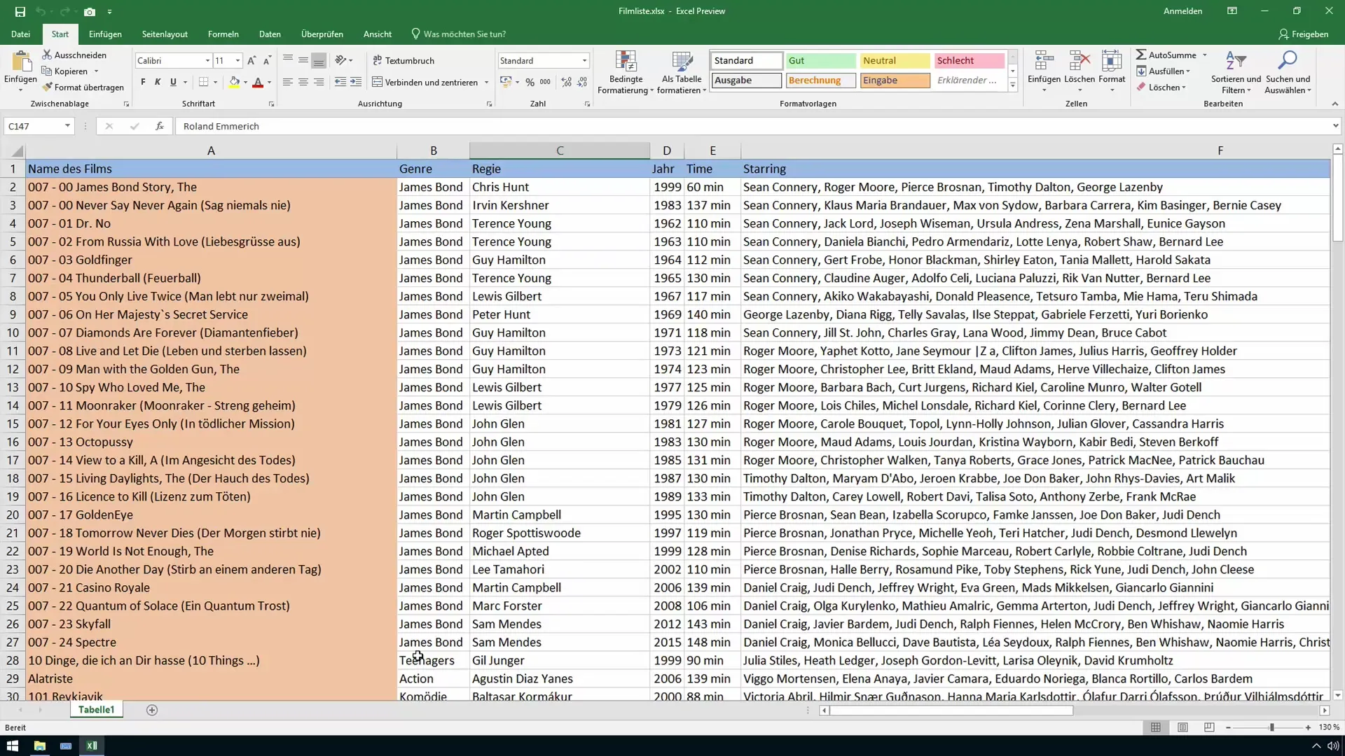
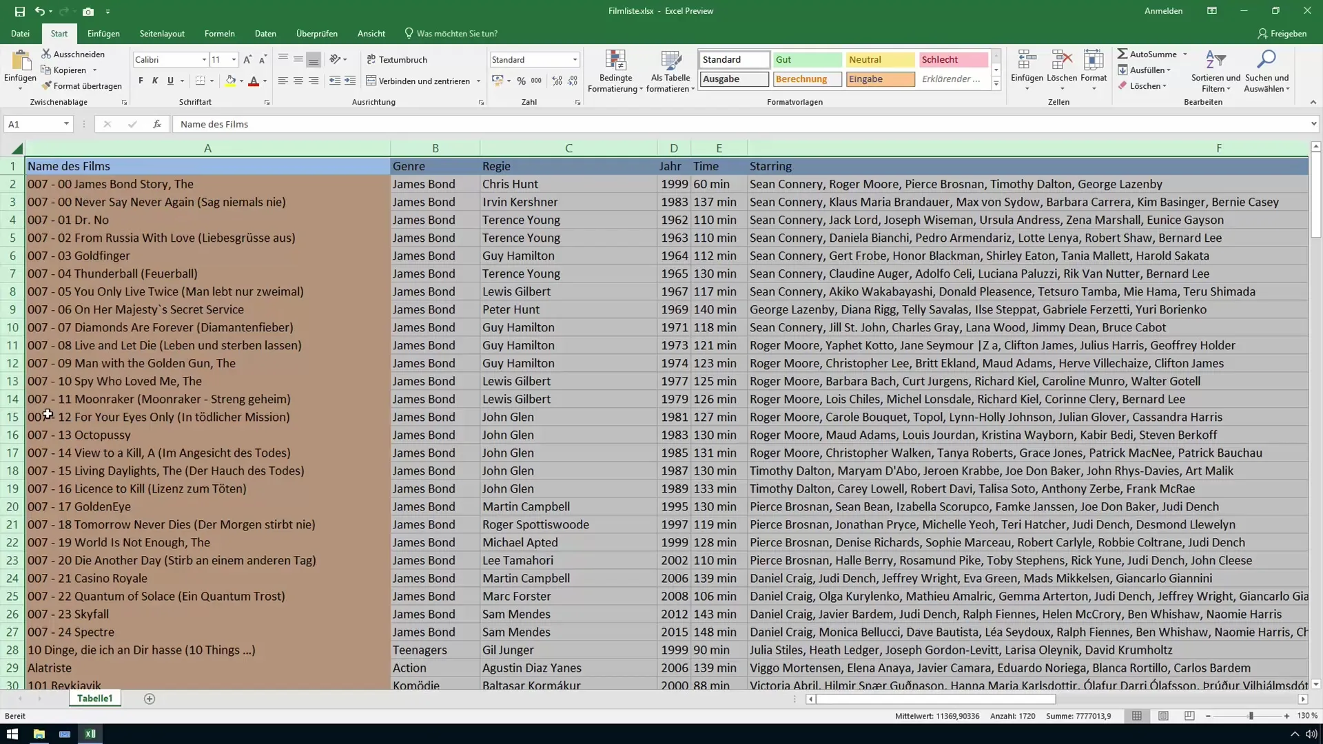
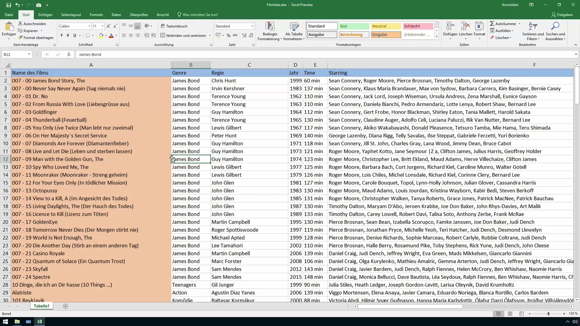
To begin, open a larger Excel table. In this case, we will use our movie list. This will allow you to easily determine which elements of the table are important to you and which are not.

In the movie list, there are many columns that may not be of interest at the moment. At this point, we are particularly interested in the movie title and the date you watched it. We can ignore all other columns, such as ratings, for now.

Select the columns you want to hide. You can use the Ctrl key or Shift key to select multiple columns at once. For example, if you do not need the columns with film details like ratings and directors, simply select them.

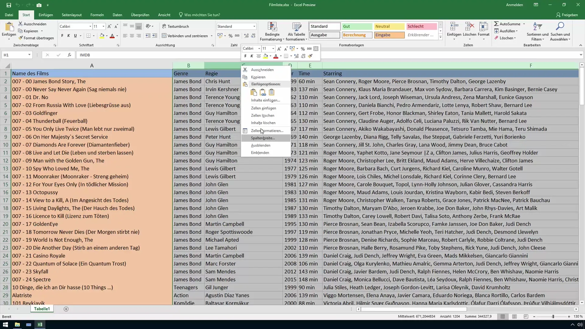
Right-click on one of the selected column headers. A context menu will open. Choose "Hide" to conceal the selected columns.

You should now see that the hidden columns between the visible columns are no longer displayed. This contributes to a better overview of your table.

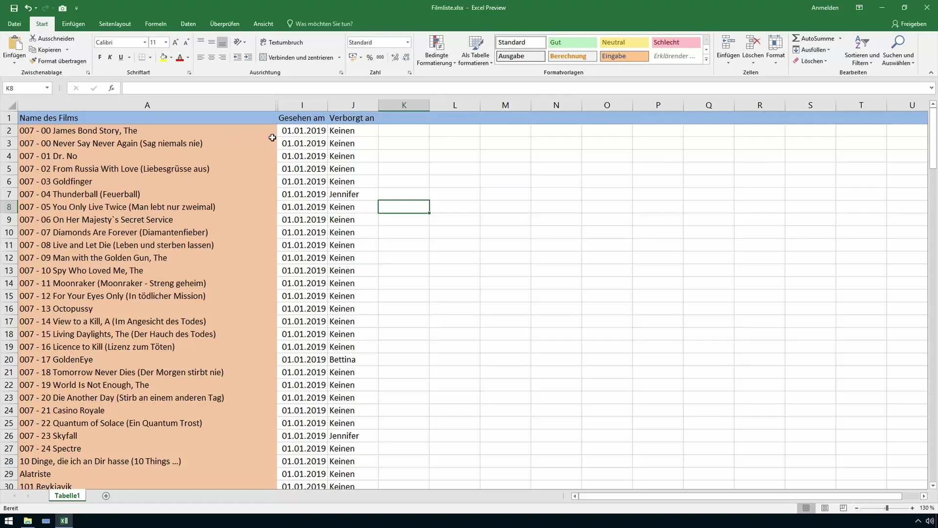
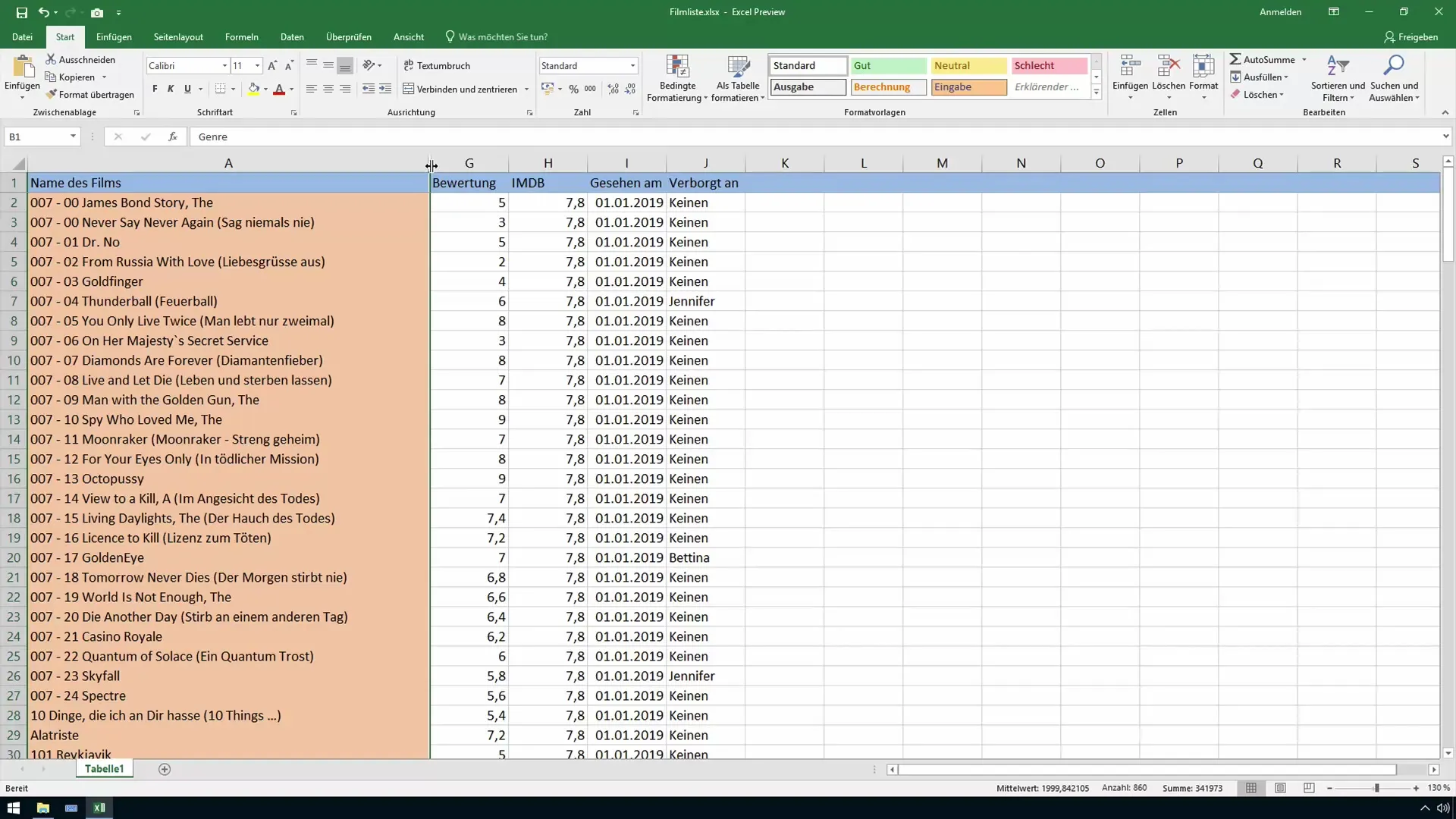
To make the hidden columns visible again, select the columns adjacent to them, as in the example columns A and I. Right-click again and choose "Unhide".

Alternatively, you can activate the unhiding function by double-clicking on the column header. Double-clicking between columns A and B will display the hidden data again, if you prefer.

The process for hiding and unhiding rows is similar. For example, if you want to hide the rows indicated by the number 007, you would proceed in the same way: select the appropriate rows and click "Hide".

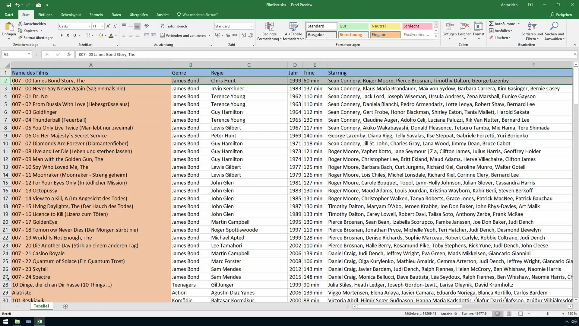
Unhiding works here as well through double-clicking or by selecting the adjacent rows and then clicking "Unhide" after a right-click.

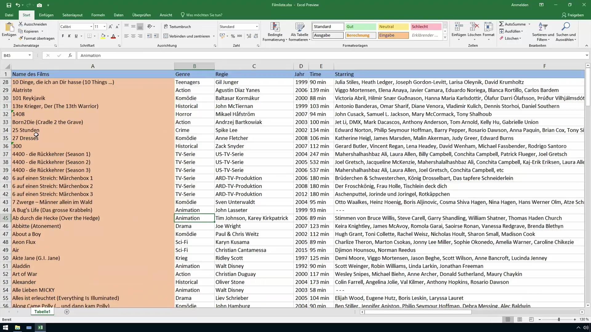
If you want to ensure that everything you hid is indeed visible again, you can select the entire worksheet and then click "Unhide". This way, you can be sure that no column or row is overlooked.

These simple steps enable you to efficiently manage your worksheets so that you only see the information relevant to your current task.

Summary

Hiding rows and columns in Excel is a simple yet effective way to increase the clarity of your data and make working with it easier. You have learned how to selectively hide data and how to display necessary information again, optimizing your Excel tables.