Effectively calculate subtotals in Excel

Excel offers numerous possibilities for data analysis and presentation. One of the most common requirements is to determine only the sums of specific cells, such as every second or fourth row. In this tutorial, I will show you how to effectively implement partial sums using array formulas.

Key Insights

• Using array formulas allows you to sum any cells in Excel.
• The combination of IF statements and the MOD function is crucial for selecting the right rows.
• You can obtain partial sums for different groups of sales data to compare performance.

Step-by-Step Guide

To understand how to sum certain cells in Excel, let's look at a concrete example where we analyze fictitious sales lists.

In this example, we are looking at a list of sales that spans from October 1st to December 31st. The task is to determine the total sum of sales and differentiate how much each seller has made.

First, you sum the sales from B2 to B93 to calculate the total sum for the quarter. This is simple and can be done using the function =SUM(B2:B93).

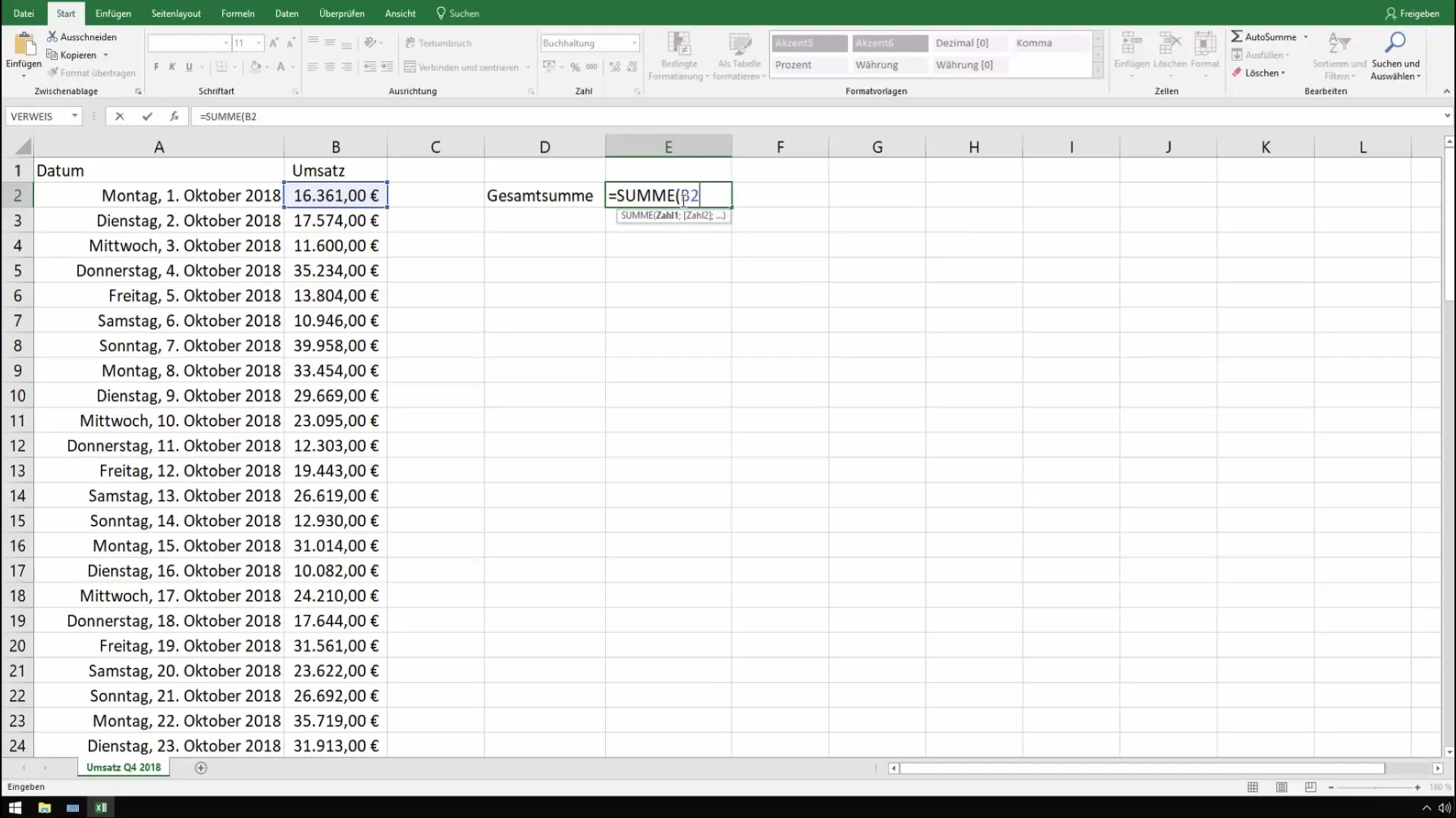
Now we want to determine the partial sum for every second or fourth day. Start by formulating an IF statement that recognizes if the current index (the row) is every second or fourth row.

Here we use the array formula to ensure that only the rows you desire are summed. We start building the sum and link it with an "IF" function to filter out the desired cells.

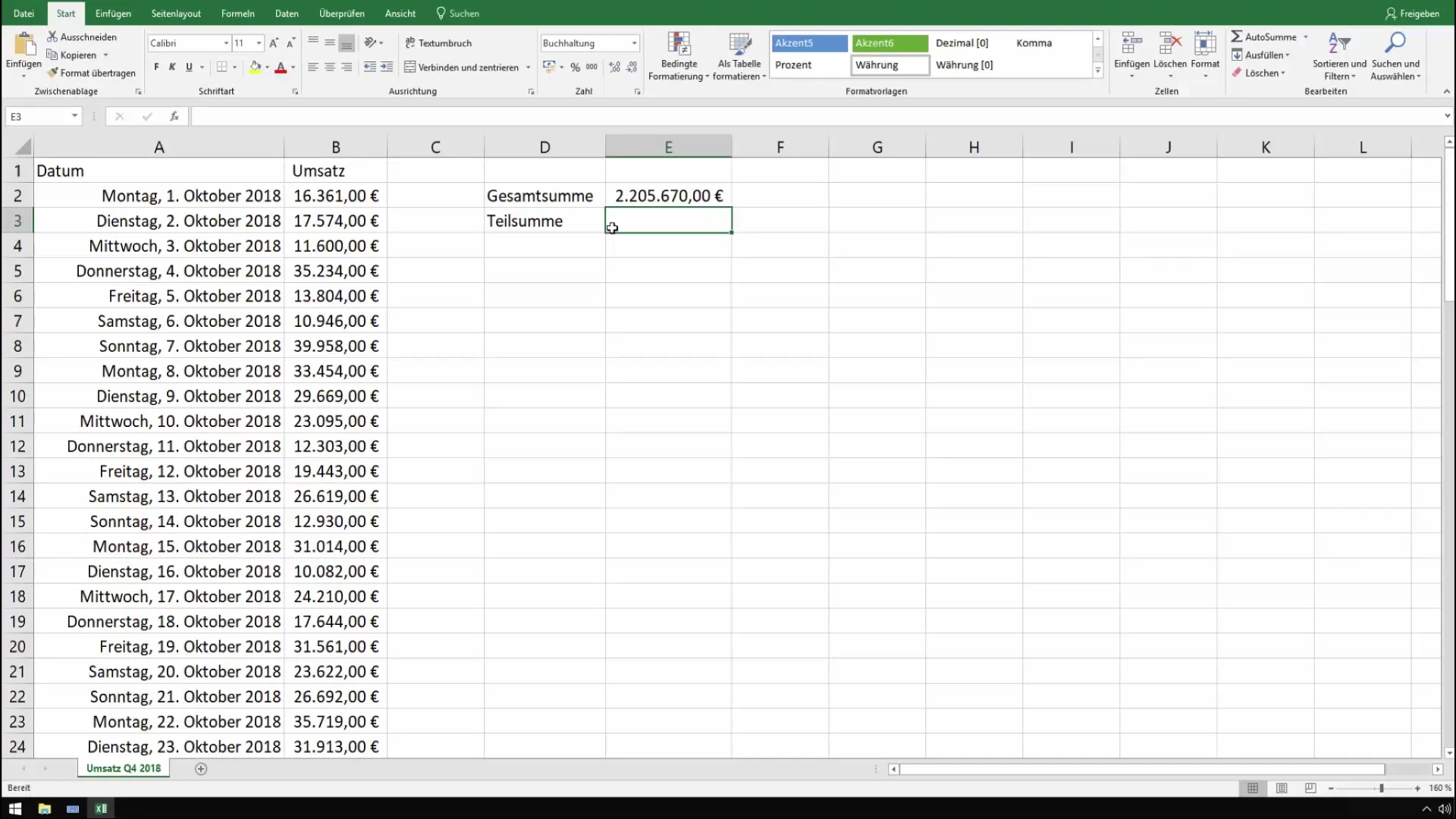
The next thing you will do is implement a truth test. This means checking if the row index is divisible by 2 (for every second day). If so, the amount should be summed.

To implement this, we use the MOD function. It allows us to calculate the remainder of a division to recognize if it is every second or fourth row, thereby creating a conditional sum.

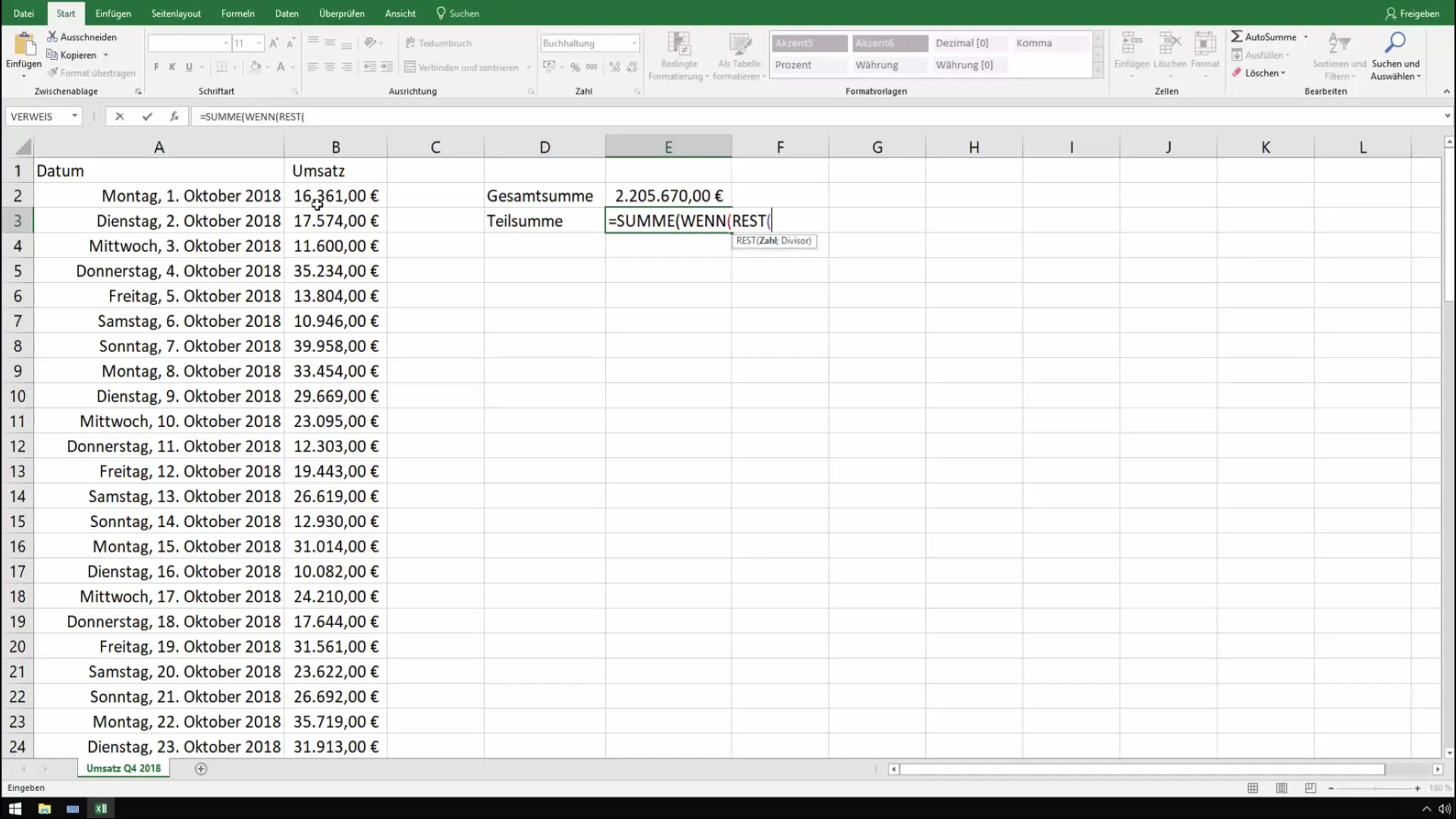
Once you have implemented the MOD function to get the remainder, you can now consider the number of rows you want to sum. Check the reference of your data to ensure you start from the right row and access the appropriate number of rows.

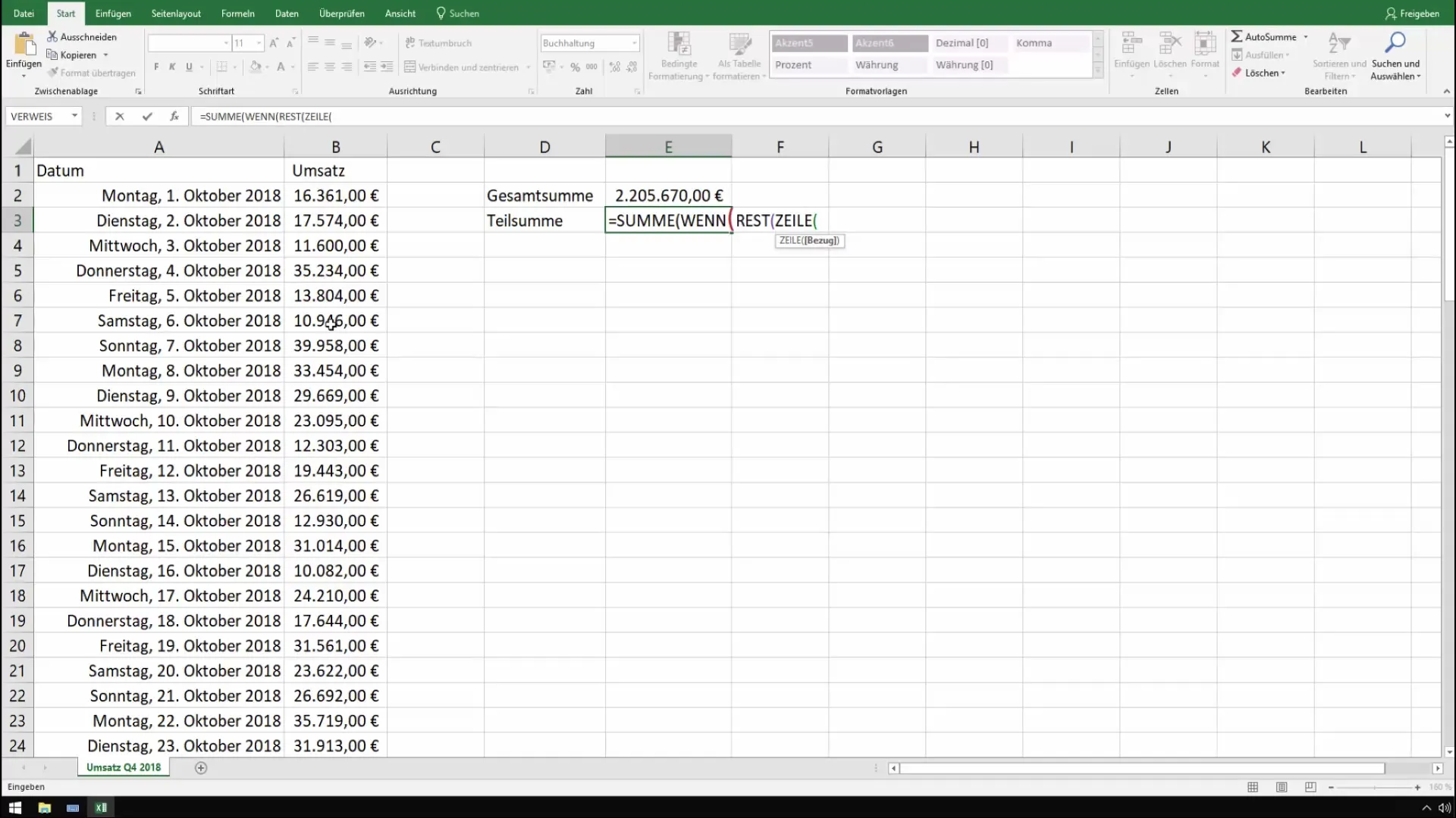
The results of your queries will display the partial sums. For example, by entering =MOD(ROW(), 2), we can find out if the current row is even or odd and adjust the sums accordingly.

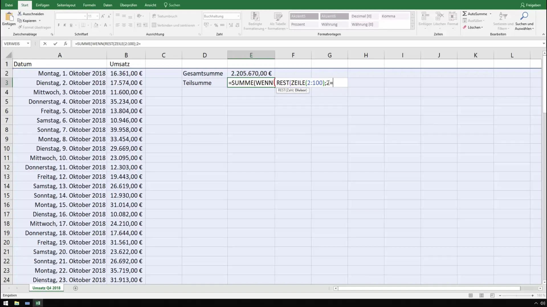
Confirm the formula with Ctrl + Shift + Enter to ensure it is an array formula. Excel will then display the output in curly brackets, indicating that the calculation was designed correctly.

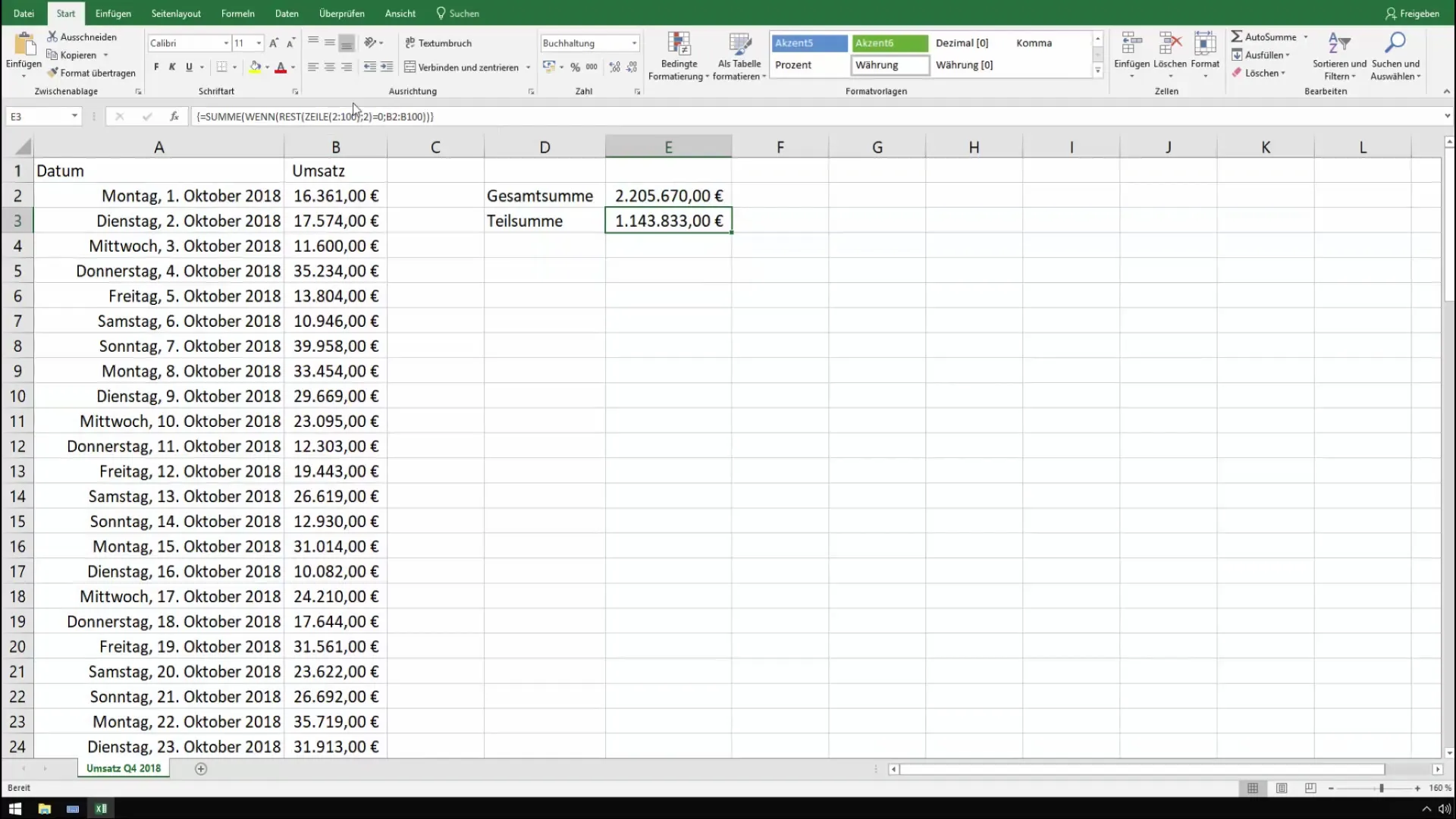
If you also want to include additional colleagues in the evaluation, you can modify the same formula and adjust it for different rows and intervals. Use relative addressing to adjust your sums without having to re-enter the entire formula.

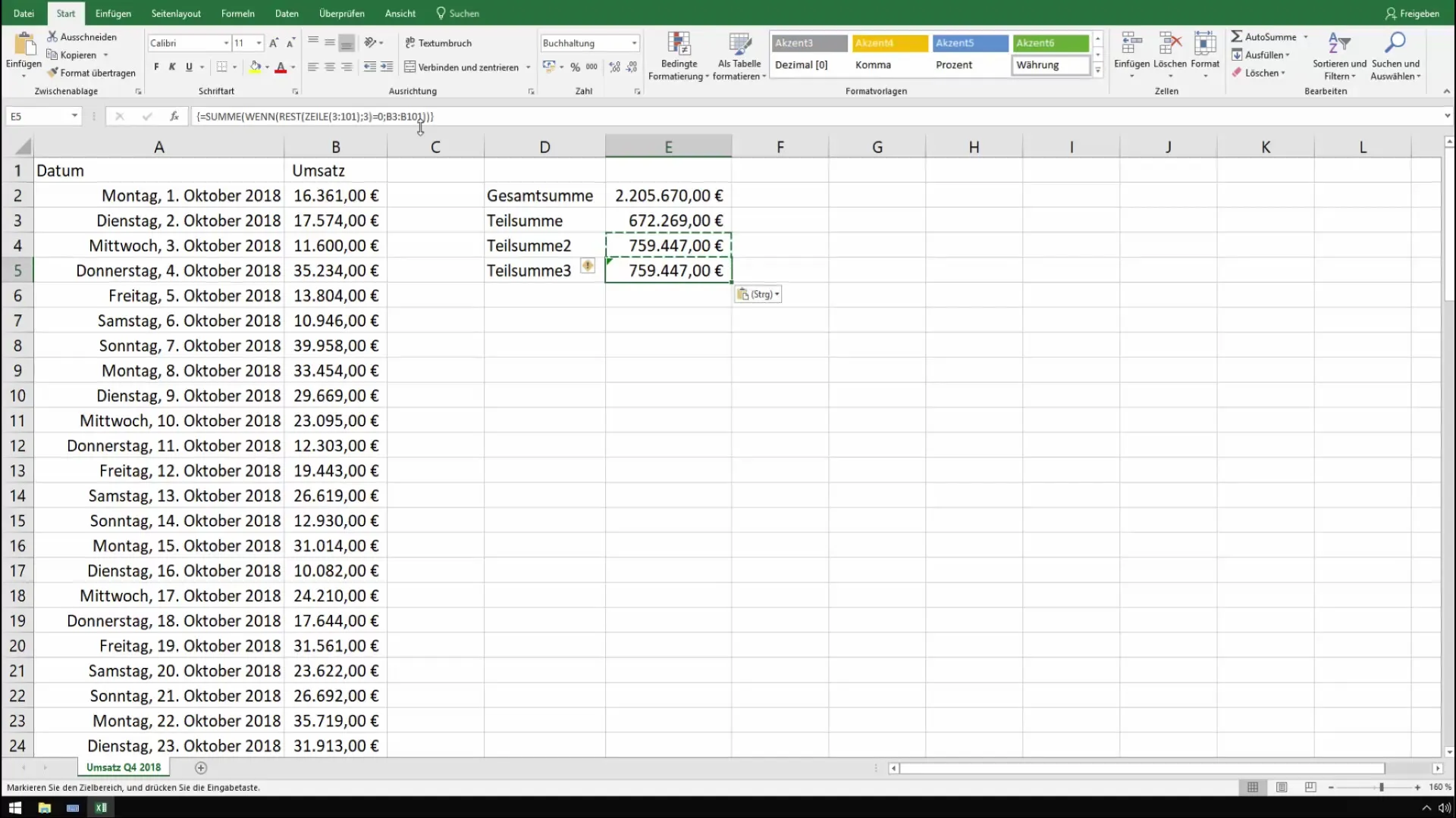
The partial sums can then be easily compared. Make sure each sum returns the correct values before presenting the final sales summary.

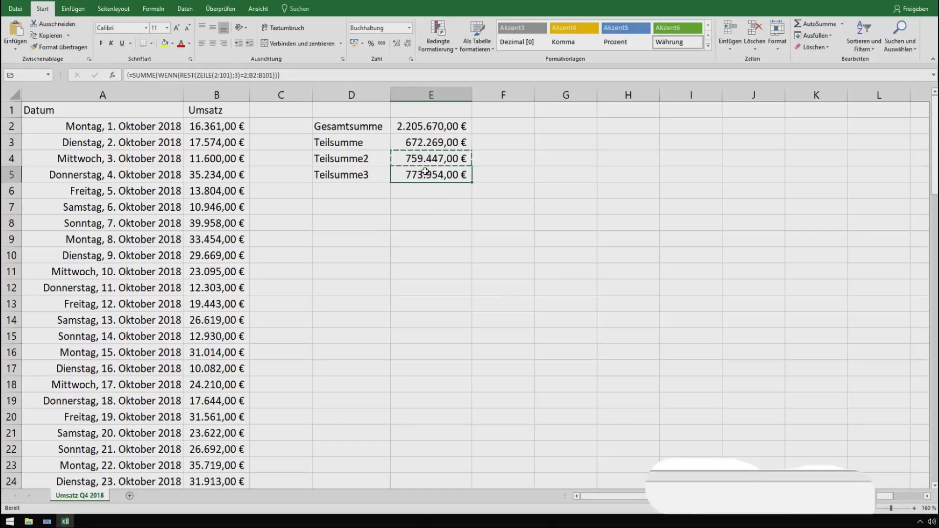
Finally, you can create a comprehensive overview of the total sums and partial sums to analyze sales performance and have the tool ready to create comprehensive reports.

Summary

In this tutorial, you have learned how to determine the subtotals of specific cells (for example, every second or third row) in Excel using array formulas. You have effectively utilized the IF and MOD functions to analyze your sales data in detail and with differentiation.