Data presentation is more than just numbers and statistics. It comes to life when the right visual cues are set. If you want to make your data more illustrative and highlight important information, conditional formatting in Excel is a great tool. With this function, for example, you can highlight weekdays in a table to make them easily recognizable at a glance. In this guide, I will show you how to apply conditional formatting for weekdays in Excel.
Key Takeaways
Conditional formatting is a versatile function in Excel that allows you to visually present data. You can highlight weekdays in a table by choosing specific colors and fonts. This makes it easier to identify patterns in data and quickly grasp important information.
Step-by-Step Guide
1. Prepare the Data
Before you start with conditional formatting, make sure you have a column with date entries in your table. Excel will only recognize these data as date values if they are in the correct format. You can use both long and short date formats.
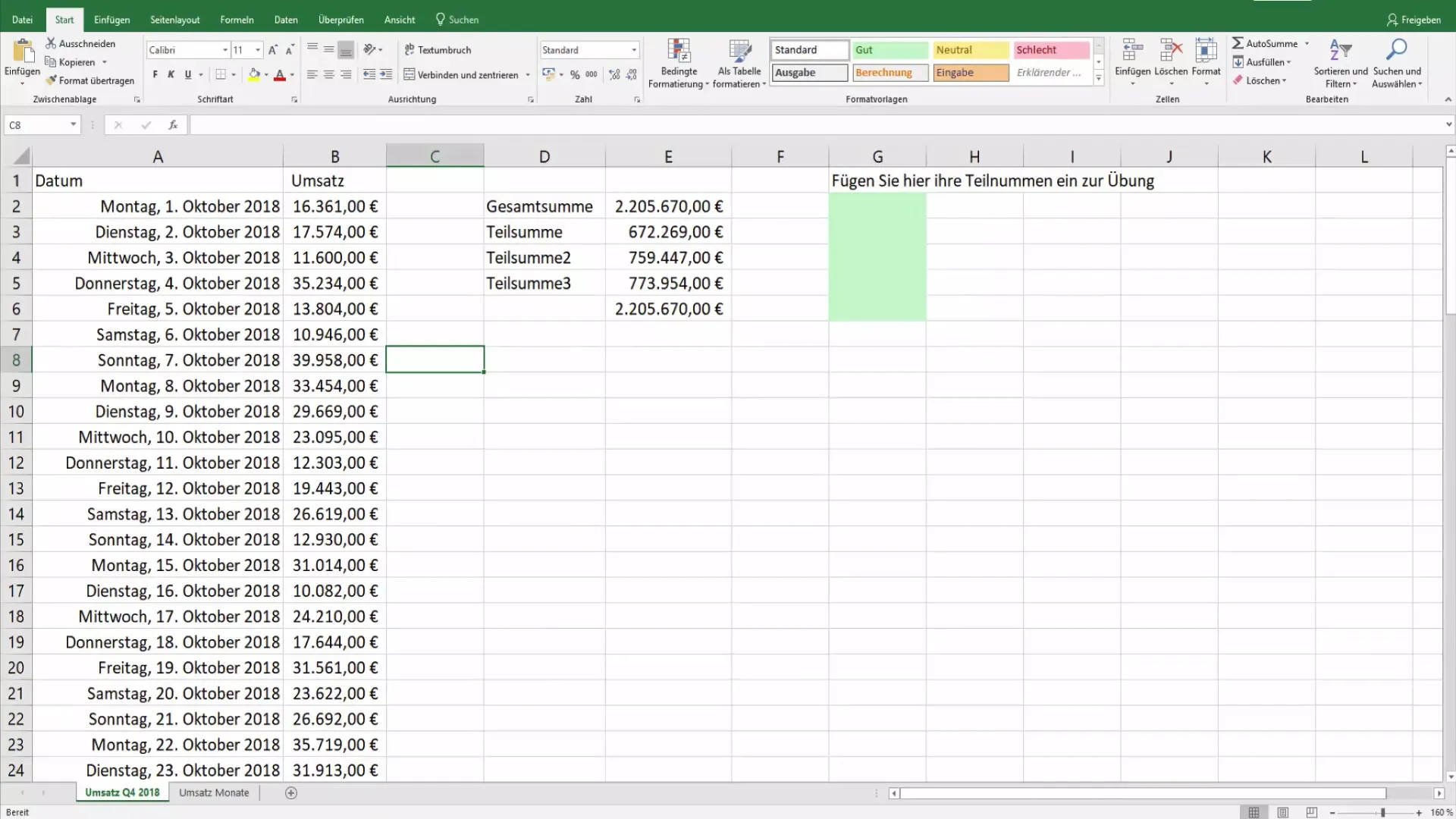
2. Select the Column
Select the entire column that contains the date entries. Click on the column to highlight it. This is the first step to applying conditional formatting to the desired cells.
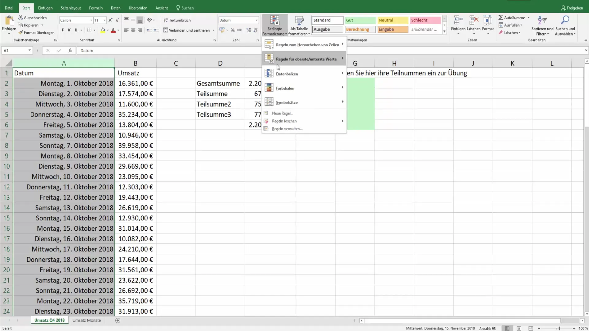
3. Open Conditional Formatting
Go to the "Home" tab in the Excel menu bar and click on "Conditional Formatting." Then choose the "New Rule" option to create a special rule to be applied to your date entries.
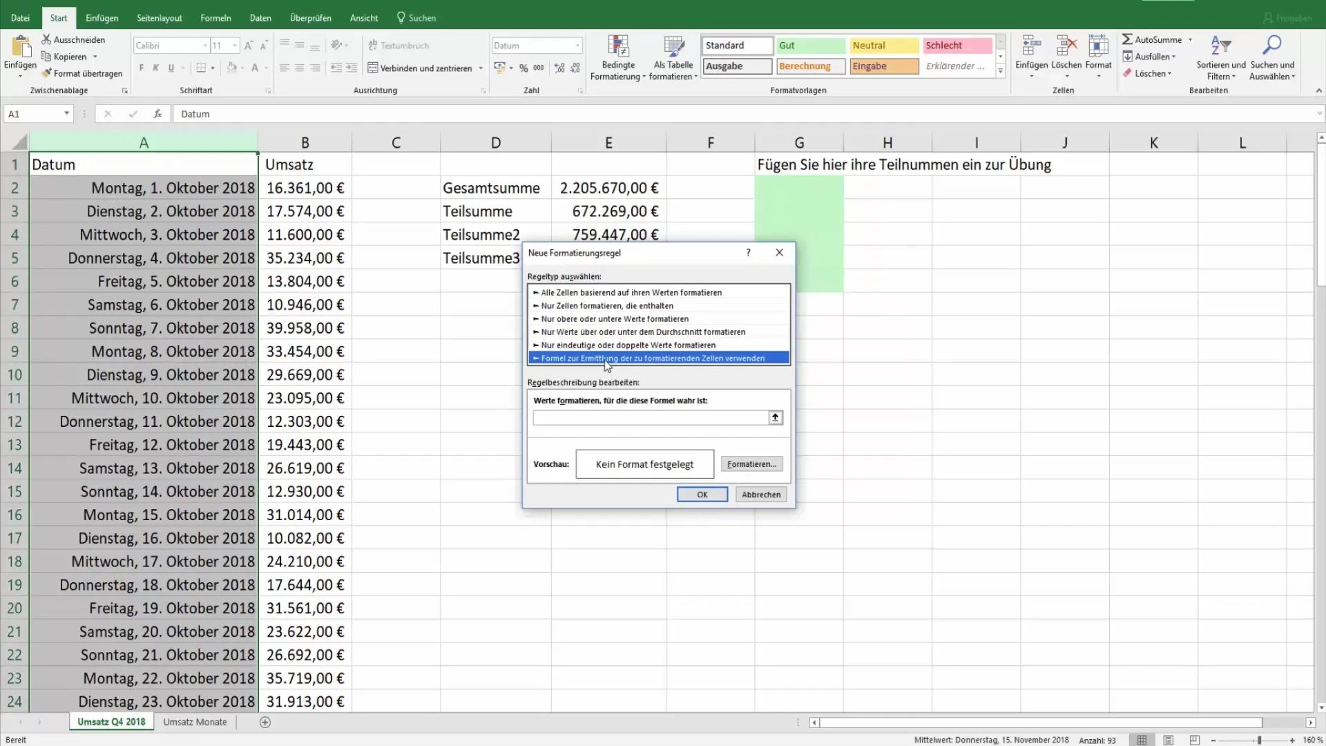
4. Select Rule Type
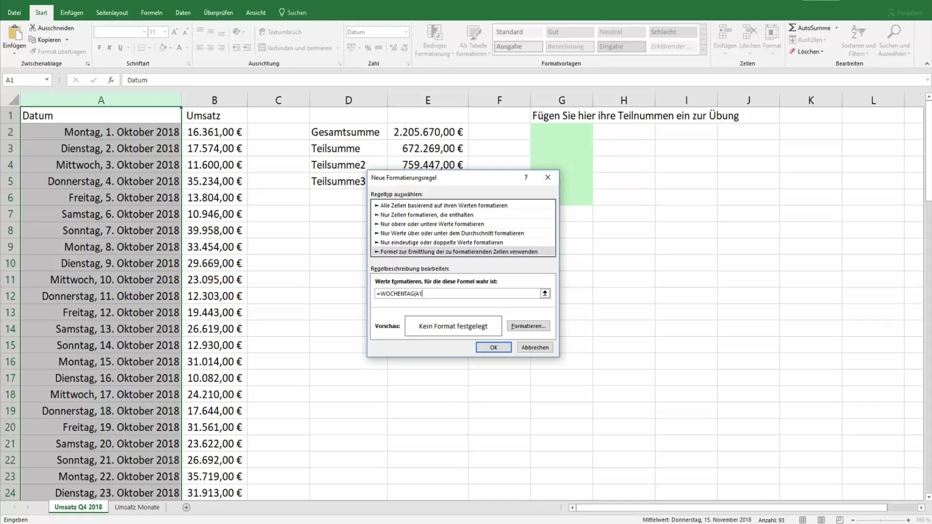
In the rules, you can choose the option "Use a formula to determine which cells to format." This allows you to use a specific formula to identify the weekdays.
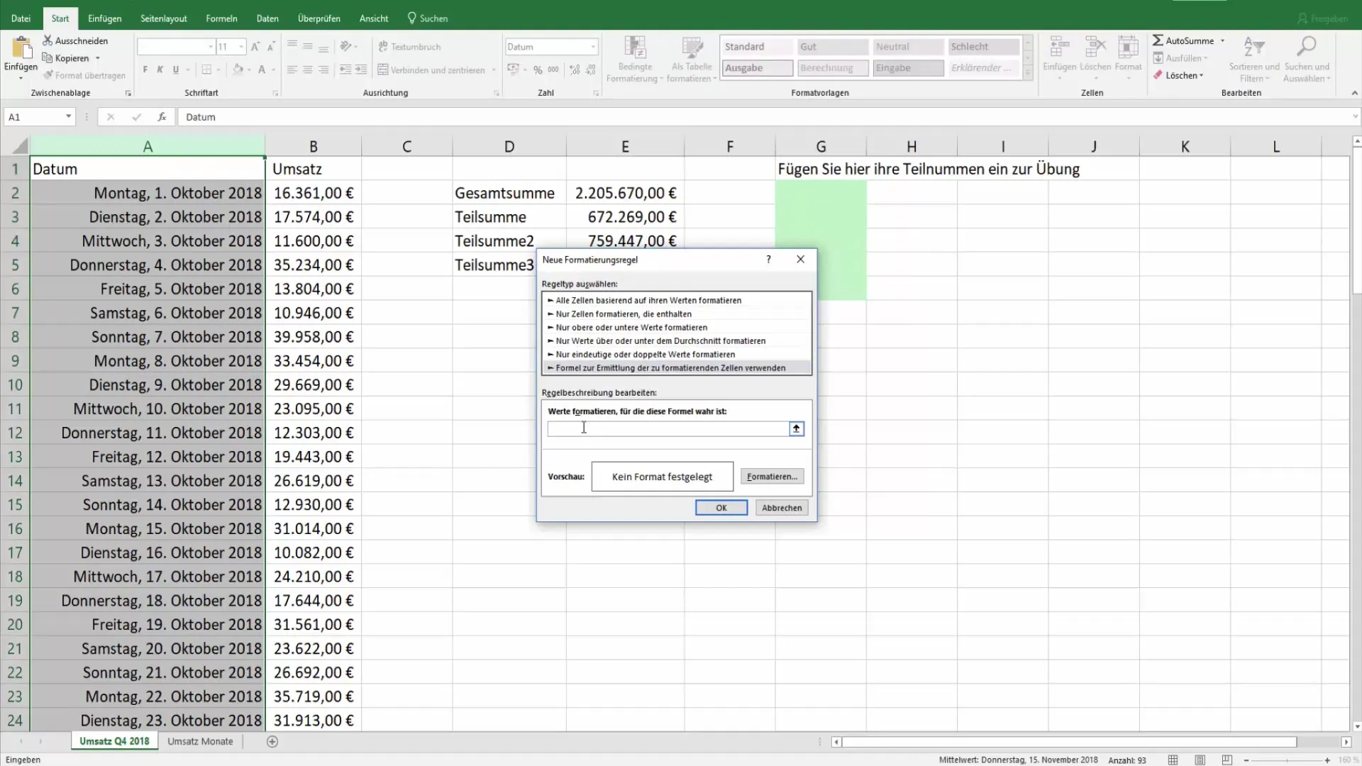
5. Enter the Formula
The next step is to enter the formula for the weekdays. Use the function "Weekday()", followed by the cell containing the date. A simple example would be: =Weekday(A1,2)>5. This formula identifies Saturdays and Sundays because they return values 6 and 7.
6. Define Formatting
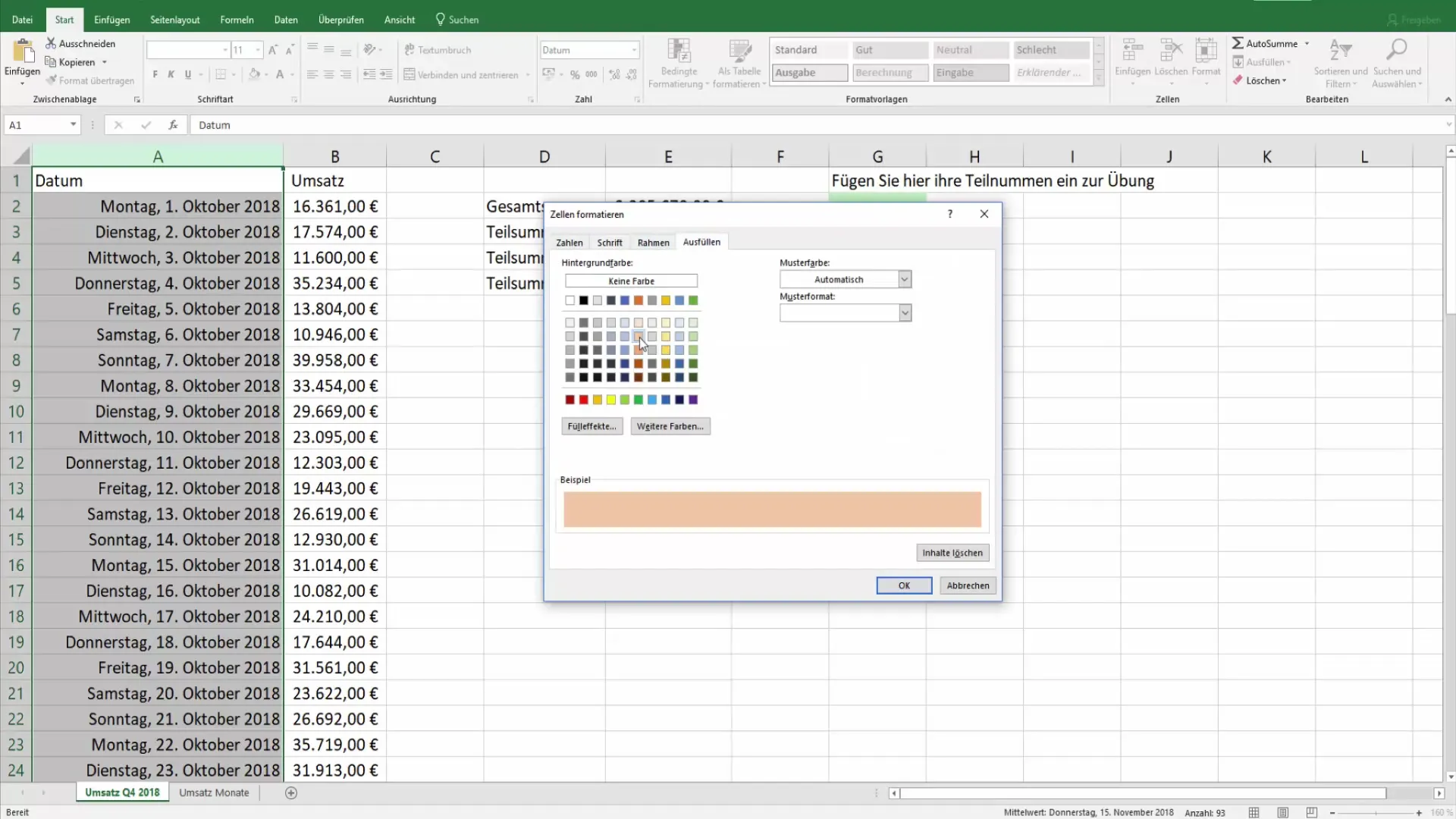
Now you need to specify how the weekends should be displayed. Click on "Format" and choose the font and colors you want to see. For example, you can format the font as bold and choose a light color like orange for the background.
7. Apply the Rule
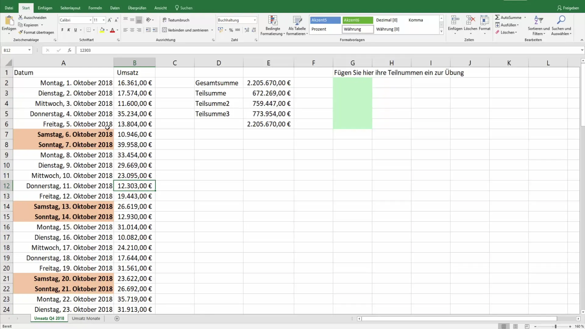
Once you have set up your formatting, click "OK" to save the rule. Excel will now apply conditional formatting to all cells in the selected column that meet the condition. This allows you to visually highlight Saturdays and Sundays and recognize them at a glance.
8. Review the Results
Review the data entries to ensure that the conditional formatting has been correctly applied. You should now be able to easily identify the weekdays. If you want to make sure everything is working, you can experiment with different date values.
9. Make Adjustments
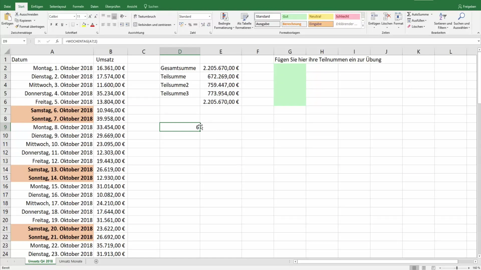
If the display does not meet your expectations, you can adjust the rule at any time. Go back to conditional formatting and edit the rule by changing the formula or formatting.
Summary
You have learned how to effectively use conditional formatting in Excel to highlight weekdays. With a simple formula and a few clicks, you can present your data more visually and emphasize important information.
Frequently Asked Questions
What is conditional formatting in Excel?Conditional formatting is a feature that allows cells to be automatically formatted based on specific conditions.
How can I color code weekdays?You can use the "Weekday()" function to identify Saturdays and Sundays and then highlight them with conditional formatting.
Can I customize the colors?Yes, you can customize the font and background color to your preference.
What happens if my date entries change?Conditional formatting updates automatically when the underlying date values change.
How many rules can I create for conditional formatting?You can create and apply multiple rules for conditional formatting in Excel.


