The presentation of data in Excel can be crucial for understandability and clarity. One of the simplest and most effective methods to visually enhance tables is to highlight rows with color. In this tutorial, you will learn how to highlight every other or even every third row in Excel with color. This is particularly useful to make large amounts of data more readable.
Key Takeaways
- There are several methods for highlighting rows in Excel with color.
- The simplest method uses Excel's built-in formatting templates.
- For more flexible adjustments, conditional formatting is recommended.
- You can not only color every other row, but also every third row to enhance clarity.
Step-by-Step Guide
Formatting rows with built-in templates
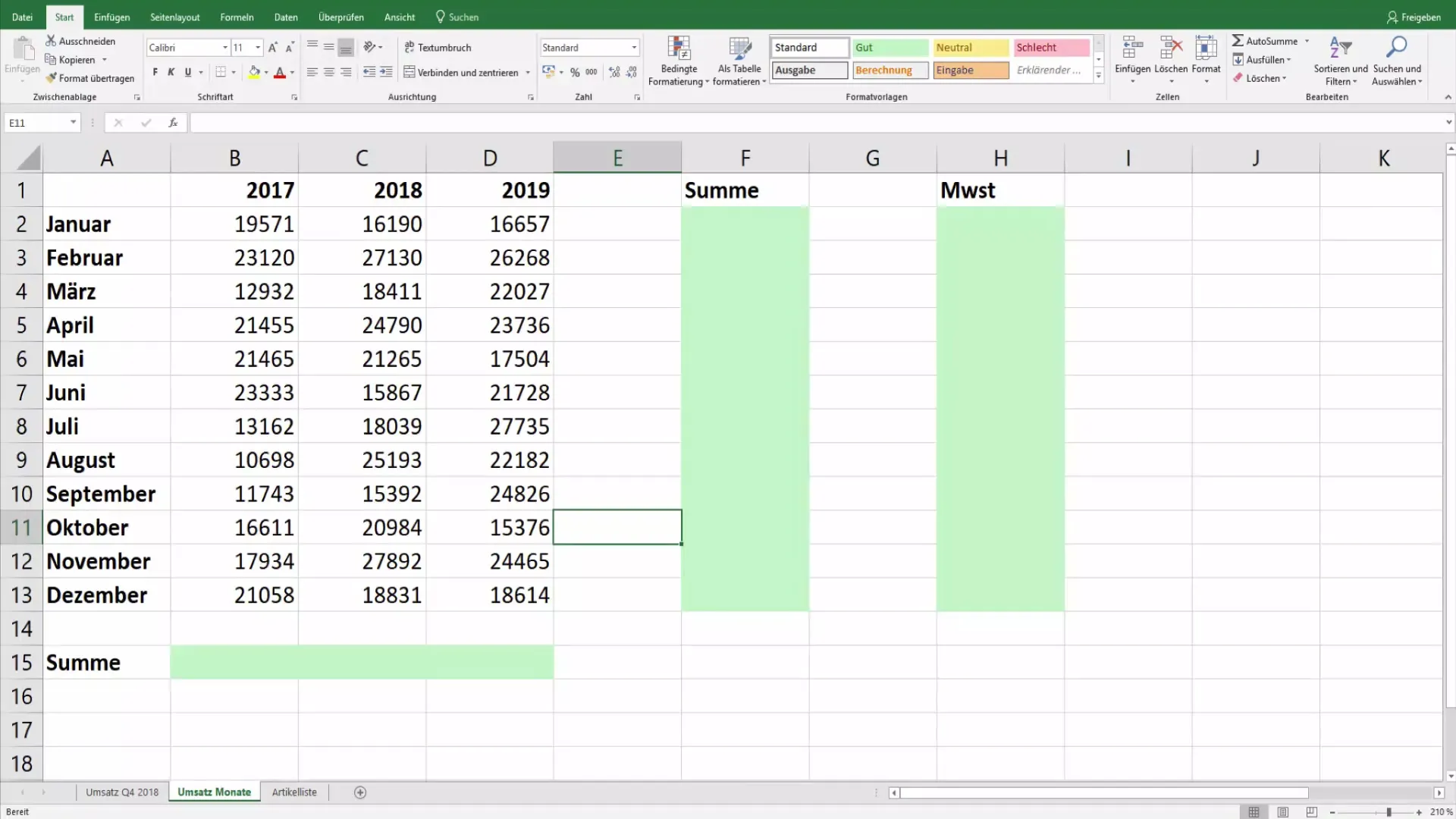
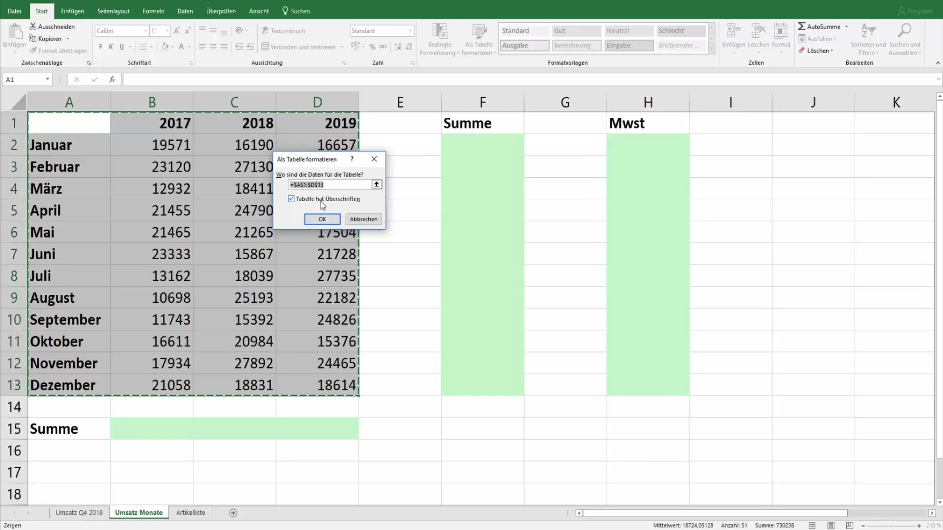
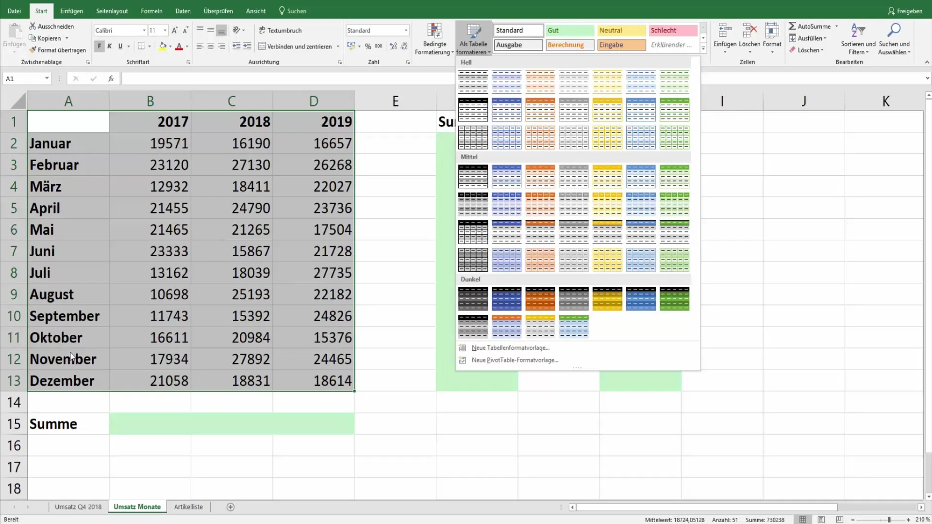
To start highlighting rows with color, select the range of your table where you want to highlight the rows with color. Then go to the "Format as Table" tab in the Excel menu at the top.
Here you will find a selection of pre-designed templates that offer a variety of color schemes. These range from different shades of gray to blue, orange, yellow, and even greenish tones. A common option is a light blue.
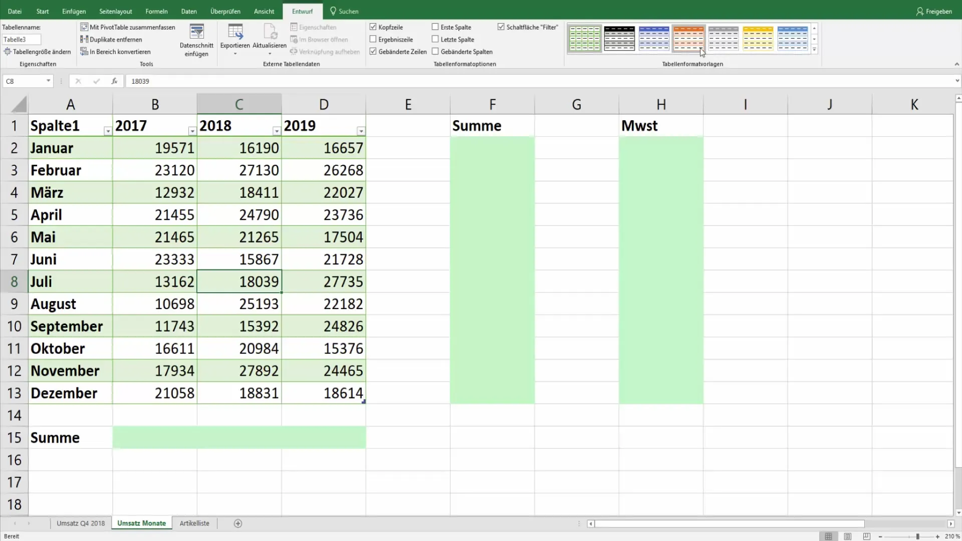
When you click on one of the templates, for example the light blue variant, your table will automatically be formatted in the chosen colors. You can decide whether the header rows should also be formatted. This way, you will immediately get an appealing and clearly structured design.
Conditional formatting for more flexibility
However, to gain more control over the color scheme of your rows, conditional formatting is the best choice. This method allows you to define specific rules. First, select the range of rows that you want to adjust the color for. Then go to "Conditional Formatting" and choose "New Rule."
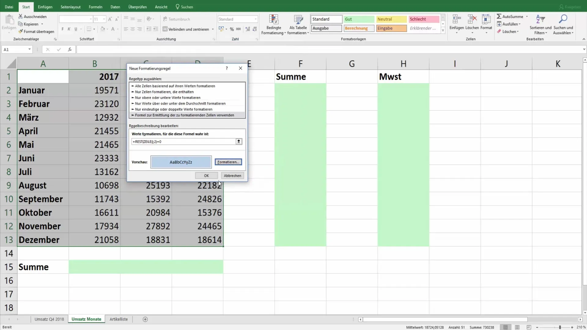
In the menu that opens, choose the option that uses a formula to determine the formatting. Here, you will use the "MOD" function. Write =MOD(ROW();2)=0 in the rule to highlight every other row.
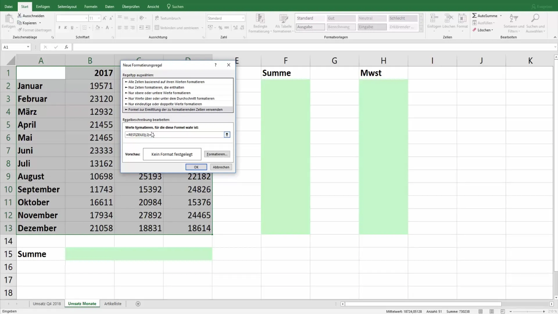
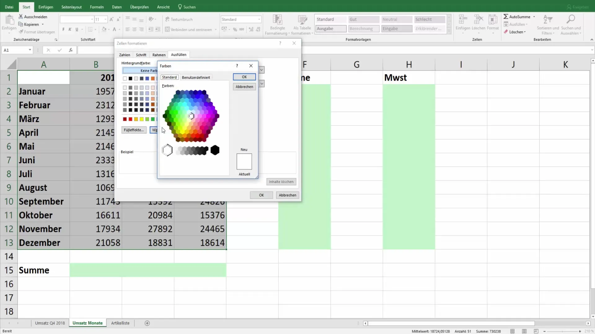
This formula divides the row number by 2 and checks if the remainder is zero. If this is the case, the formatting is applied. You can make further adjustments by clicking on the "Format" button and selecting the desired fill color.
Colorful styling of every third row
If you also want to highlight every third row with color, create a new rule. Here you can follow the same steps again and use the formula =MOD(ROW();3)=0. This rule will format the rows where the row number, when divided by 3, has a remainder of zero.
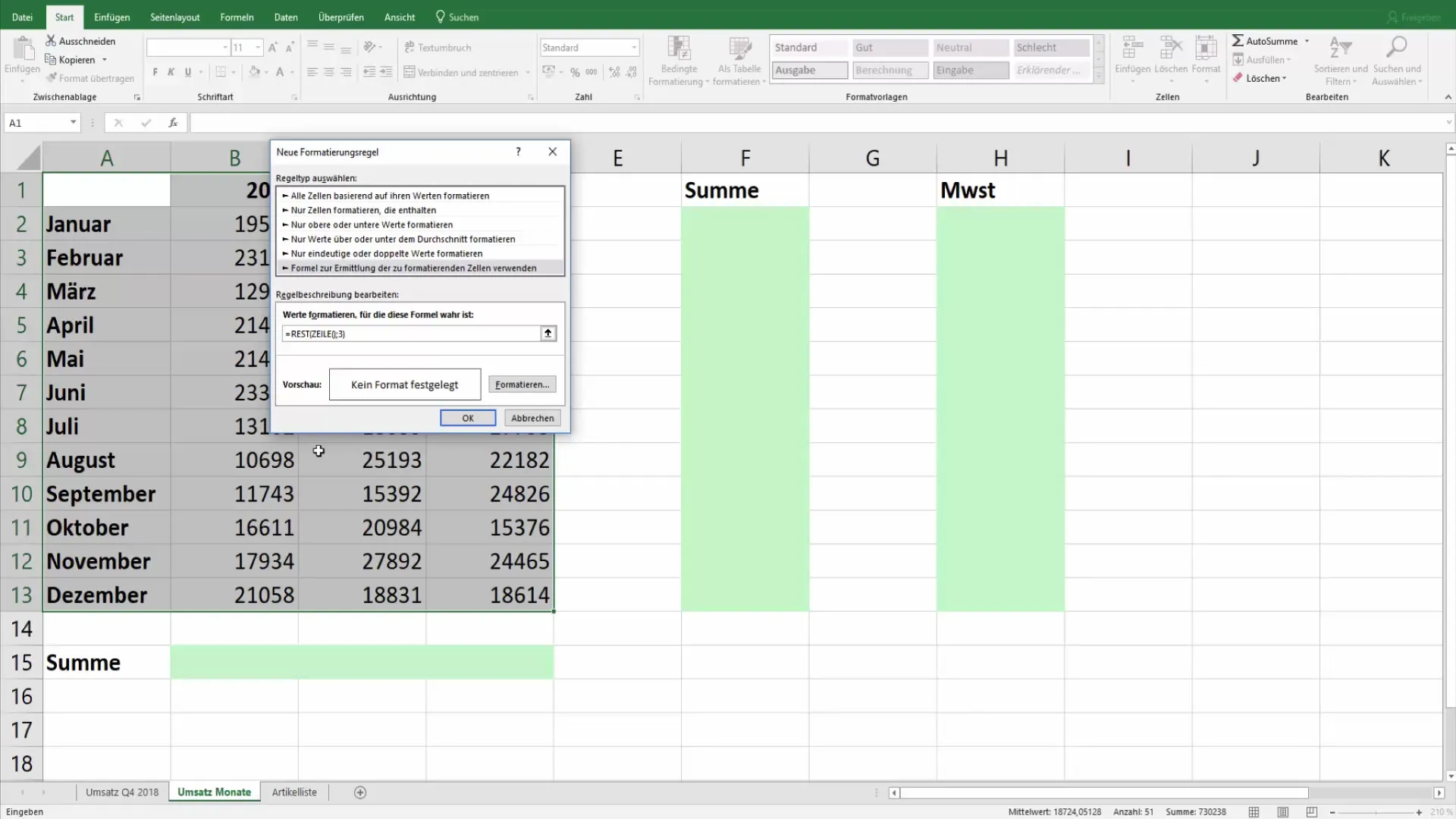
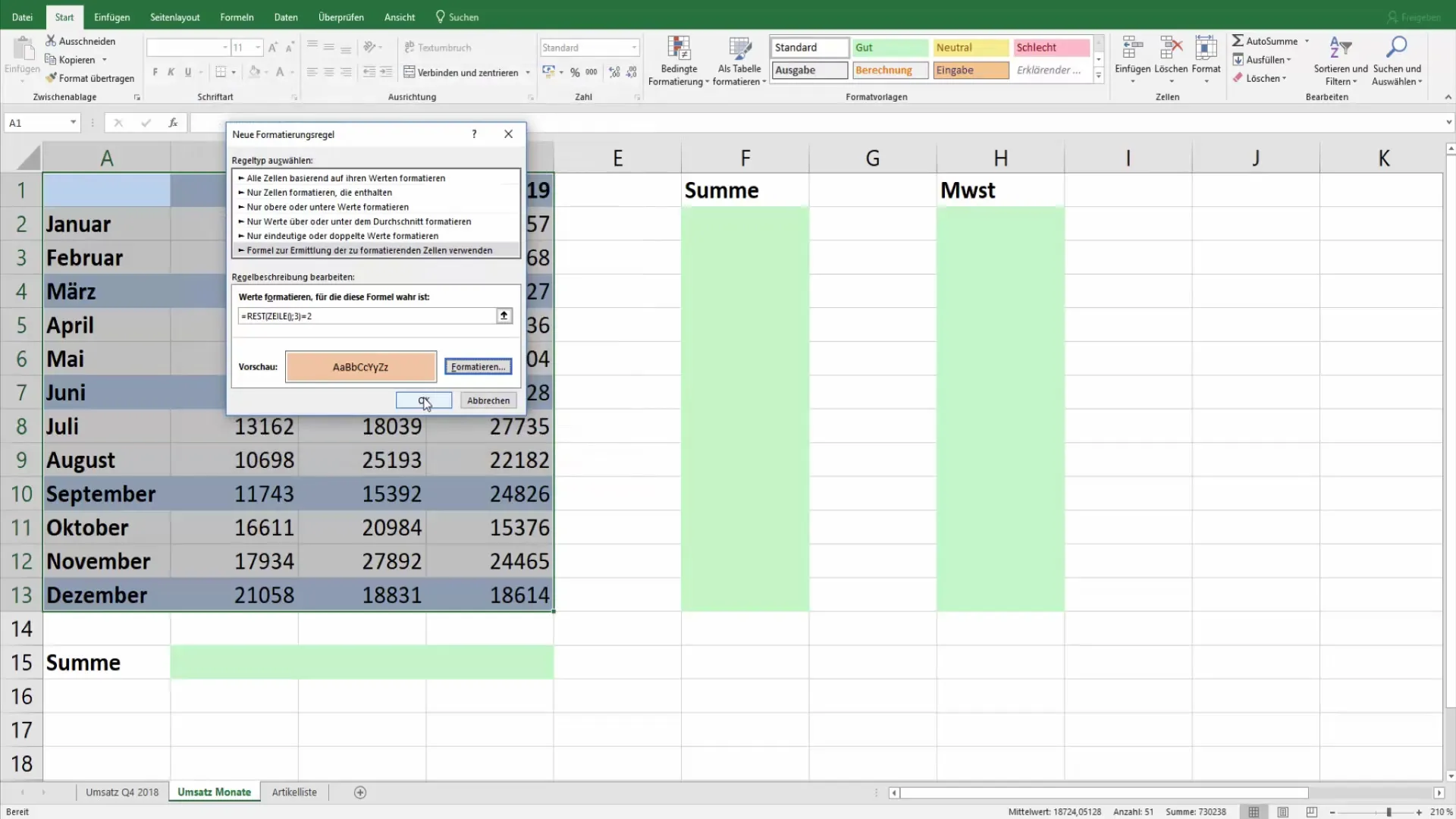
You can create additional rules to apply different colors to different rows. Set the rule for remainder 1 and remainder 2 for added color variations. For example, you can set the color for remainder 1 to light blue and for remainder 2 to orange. This way, you assign different colors to your rows, creating a clear separation.
Ensuring consistency
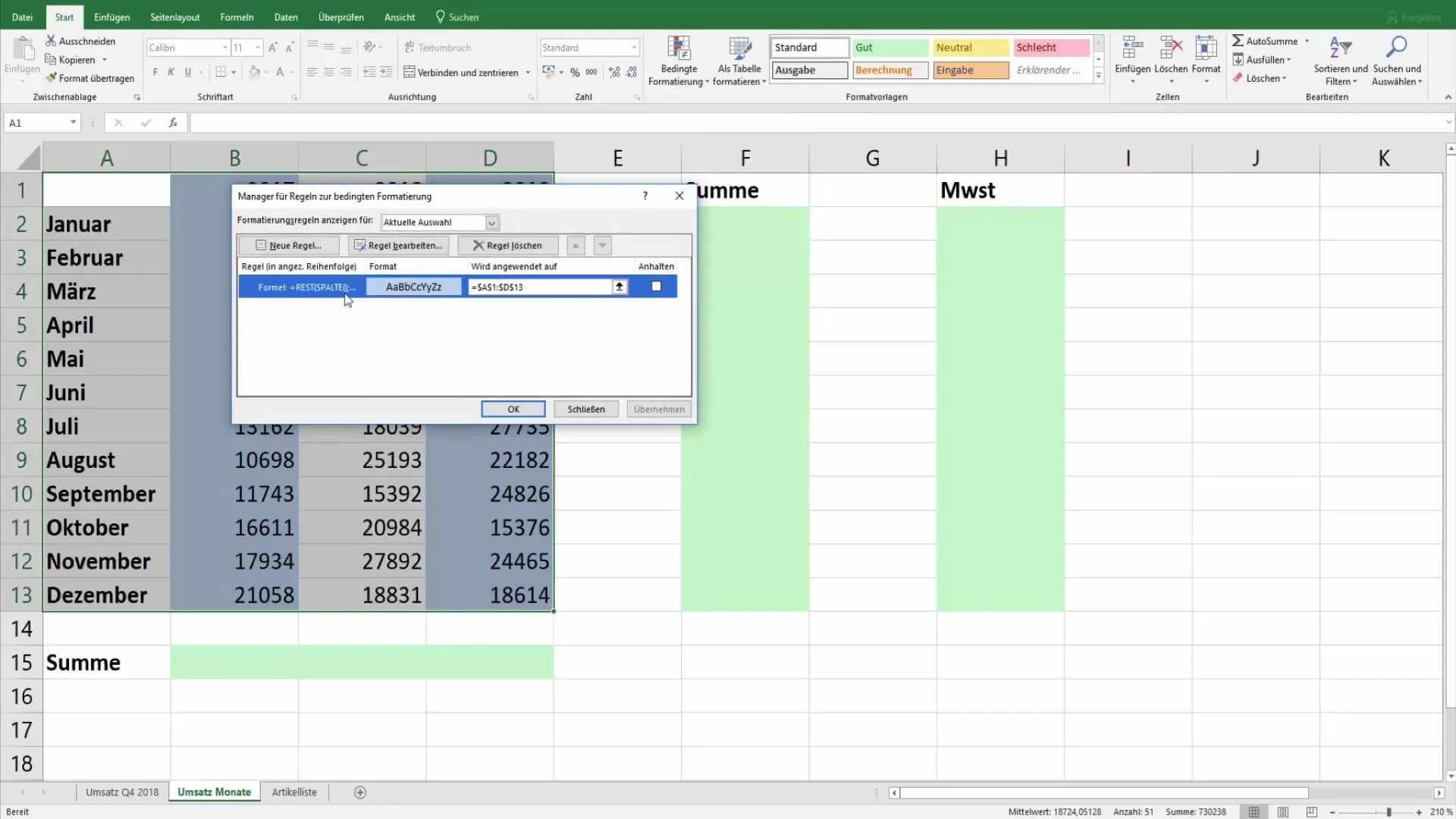
If you notice that the desired formatting is not working as planned, you can check in the rule management which rules are active. Here you can delete or edit rules that are no longer needed to restore your desired formatting.
Fine-Tuning the Colors
Another tip is that when formatting your rows, you also have additional colors to choose from. Standard colors are often nice, but customizing to fit your preferences can help personalize a table that better suits your needs.
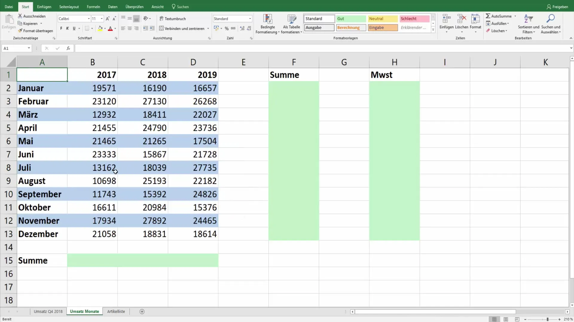
If you want to ensure the changes and check the formatting, simply test your table by adding some fictitious data to see if the formatting is applied correctly.
Summary
In this tutorial, you have learned how to highlight every second and third row in color in Excel. You have discovered different methods, starting from pre-defined formats to conditional formatting, which offers you the flexibility to define different rules. These techniques enhance the readability of your data and make your tables visually appealing.
Frequently Asked Questions
How can I highlight every second row in Excel?Use conditional formatting with the formula =MOD(ROW(),2)=0.
Can I also highlight every third row in color?Yes, simply use the formula =MOD(ROW(),3)=0 in conditional formatting.
How can I customize the colors?Click on "Format" in the rule management and choose from a wide color palette the desired colors.
Can I apply multiple color rules for different rows?Yes, you can create multiple rules and set different colors for different remainder values.
What to do if the formatting is not displayed correctly?Check the rule management and make sure that the correct rules are active, or delete unnecessary rules.


