Excel status bar - quick calculations made easy

Excel is not just a tool for creating tables and charts, but it offers numerous possibilities to optimize working with data. One often overlooked feature is the status bar, located at the bottom of the Excel interface. In this guide, you will learn how to effectively utilize the potential of the status bar to perform calculations with just a few clicks and keep track of your numbers.

Key Insights

• The status bar allows quick calculations like sum, average, minimum, and maximum.
• You can customize the values displayed on the status bar to make the most important information visible to you.
• You can check results quickly without using formulas and complex functions with the status bar.

Step-by-Step Guide

1. Finding the Status Bar

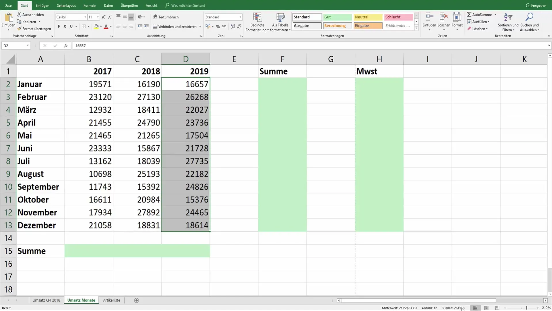
To start working with Excel, you first need to find the status bar. It is located at the very bottom of the Excel window. The status bar is often referred to as a small calculator as it offers many useful functions to help you quickly analyze data.

2. Selecting Numbers

To perform calculations, select the numbers you want to work with. You can simply click and drag to select the desired cells. For example, if you have a list of sales figures, select them to analyze them in the status bar.

3. Checking Results in the Status Bar

Once you have selected the numbers, you will immediately see the sum of the selected values in the status bar. This happens automatically, so in most cases, you do not need to enter formulas. You will get a real-time overview of the relevant calculations, saving you time and effort.

4. Displaying Additional Calculations

In addition to the sum, you can also display the average and the number of selected cells in the status bar. These values provide important information about your data without additional steps or calculations. To see the number of selected cells, simply look at the status bar after selecting the cells.

5. Context Menu for Additional Options

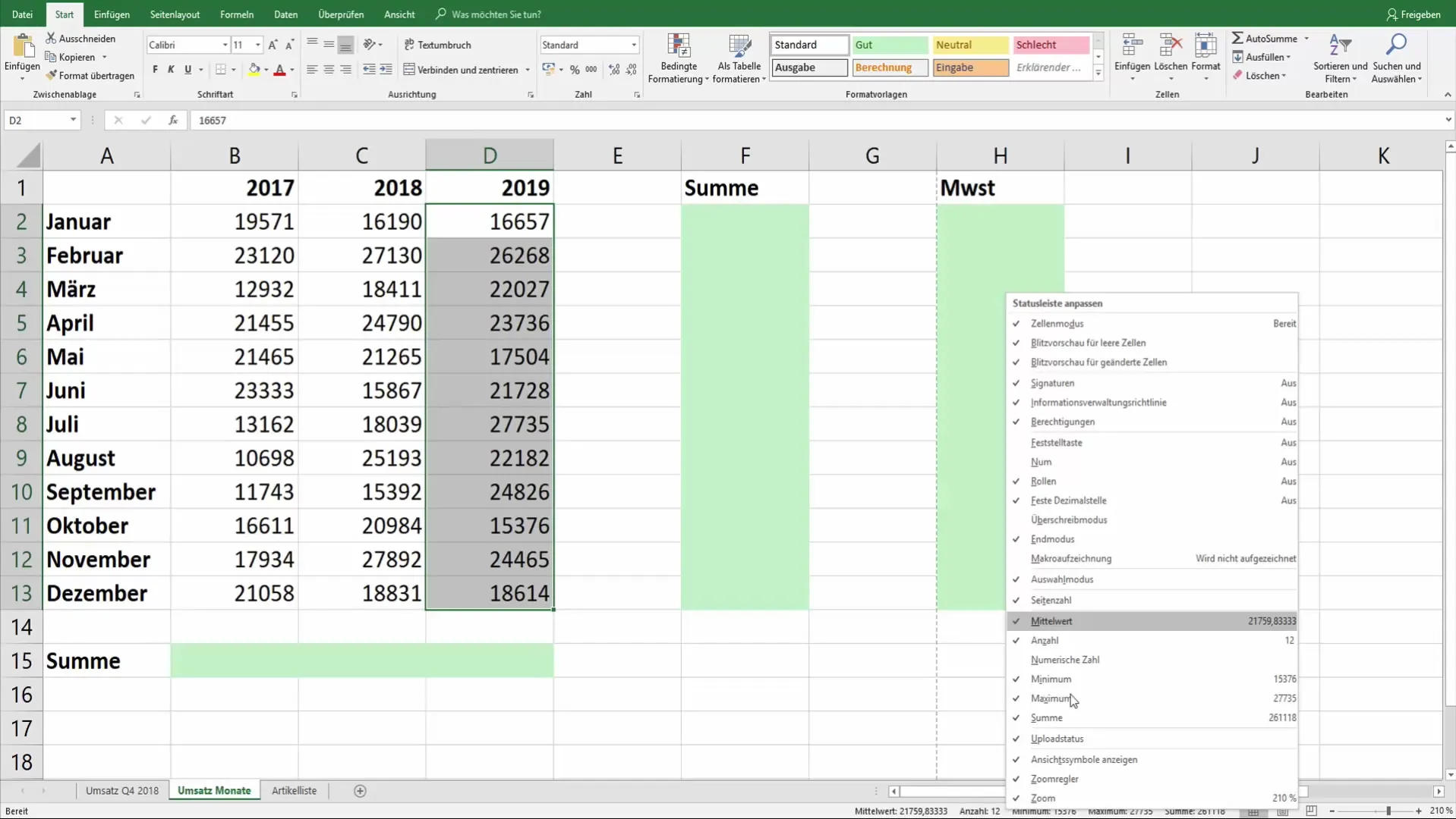
By right-clicking on the status bar, you can activate additional calculations like minimum and maximum. These options offer more flexibility, allowing you to see the information most relevant to your tasks. You can easily switch between these options to better understand your data.

6. Analyzing Key Values

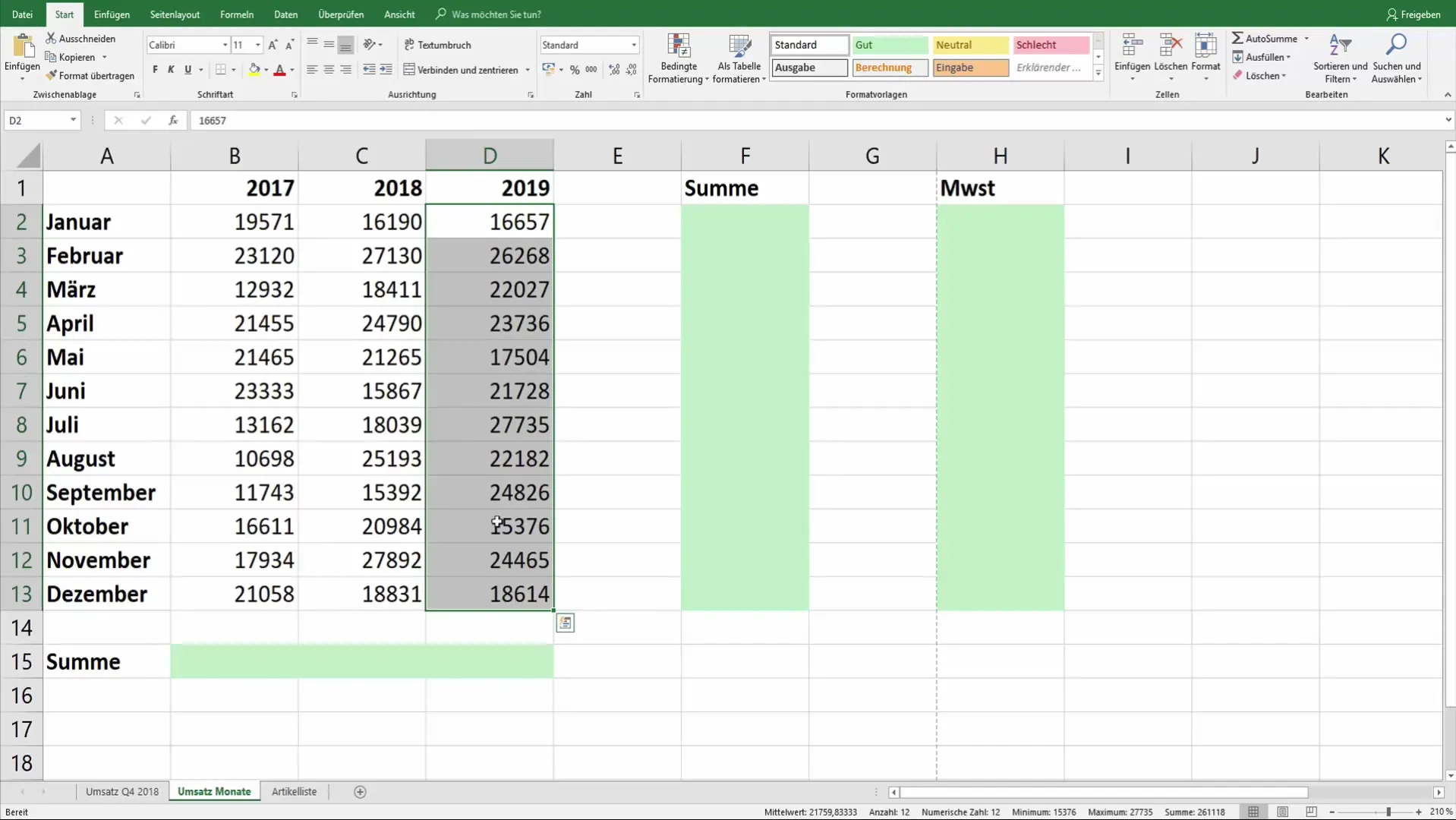
Now you should have a good overview of the key values in your selected data. For example, the minimum of the selected values is crucial to ensure that there are no outliers in your data. Here you have the values, such as minimum 15,376 and maximum 27,735, readily available for quick analysis.

7. Interpreting Results

Use the displayed results in the status bar to check and interpret your data. When you see the sum, minimum, and maximum at a glance, you can make decisions faster and identify issues in your data.

8. Conclusion on Using the Status Bar

In conclusion, the status bar in Excel is a powerful tool that helps you perform the most important calculations quickly and efficiently. You do not need to use formulas to obtain simple statistics. The functionality is ideal for quick checks and data analysis.

Summary

In this guide, you have learned how to effectively use the status bar in Excel to quickly perform calculations like sum, average, minimum, and maximum. The ability to easily select cells and see instant results makes Excel an even more powerful tool for your data analysis.