If you want to analyze and present your data in Excel, using functions for targeted summarization is essential. The "SUMIF" function in particular helps you apply specific criteria and sum only the desired values. In this tutorial, you will learn how to effectively use the "SUMIF" function to sum the desired data and make your evaluations directly in an Excel table.
Key Takeaways
- The "SUMIF" function can be used to sum only the values that meet certain criteria.
- Correct syntax is crucial for success, where the search range and sum range must be clearly defined.
- Wildcards such as a question mark and asterisk can be used to define flexible search criteria.
Step-by-step guide
Example with Condominiums
You start with a list of condominiums and want to sum the commissions for properties that exceed a certain value.
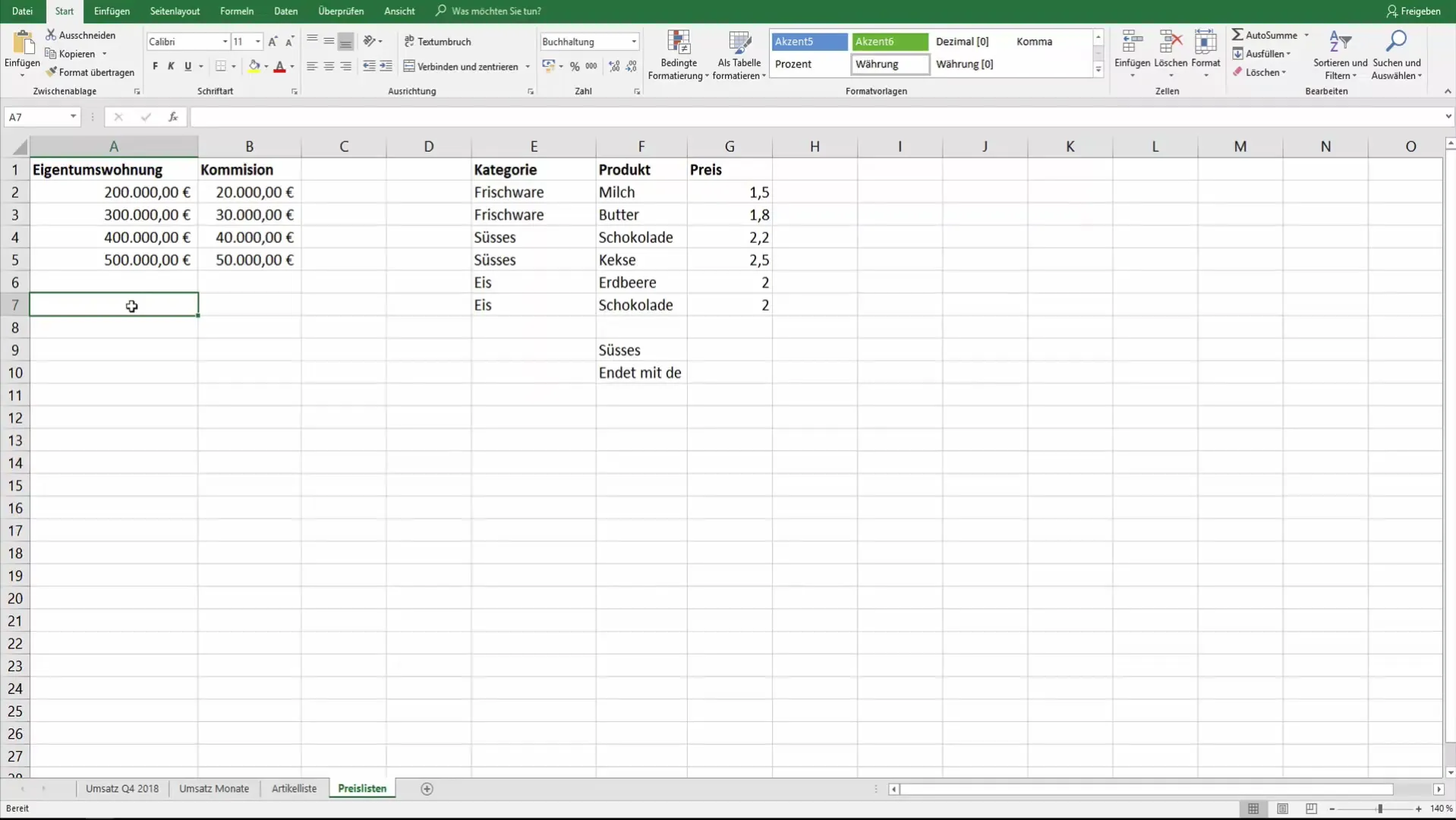
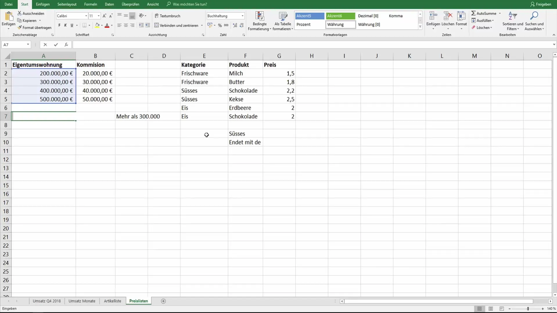
First, you define the data in your Excel table. You have a column with the values of the condominiums (e.g., €200,000, €300,000, €400,000, €500,000) and another column with the corresponding commissions (e.g., 10% of the property prices).
To sum the commissions of condominiums that cost more than €300,000, you use the "SUMIF" function. To do this, select the range of property prices as the search range. This could range, for example, from cell A2 to A5.
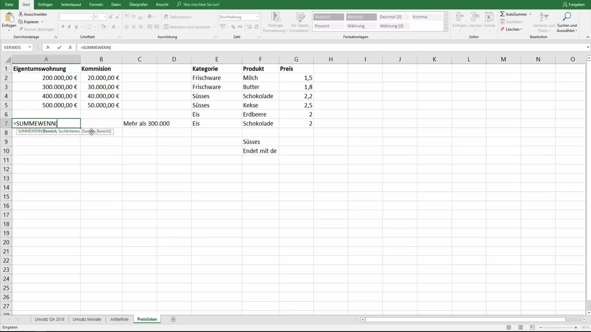
Now you insert the function: =SUMIF(A2:A5, ">300000", B2:B5). Here, A2:A5 represents the search range, ">300000" is your criterion, and B2:B5 is the sum range where the commission amounts are listed.
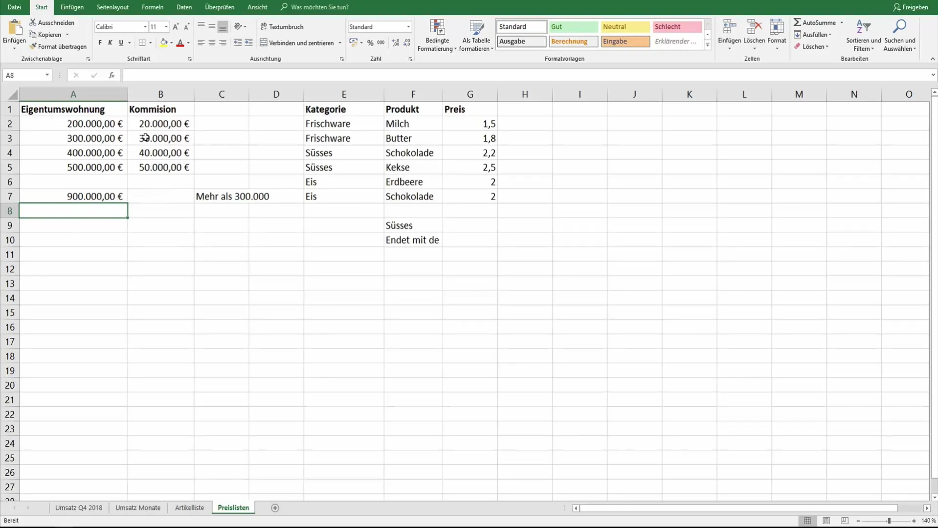
Press Enter, and Excel will calculate the sum of the commissions for all properties valued over €300,000. The result should be €90,000 if the commissions are €40,000 for the €400,000 property and €50,000 for the €500,000 property.
Example with Different Product Categories
Another practical example is analyzing different product categories in a supermarket. Here, the focus is on determining the total sum for products in a category, such as "Sweets."
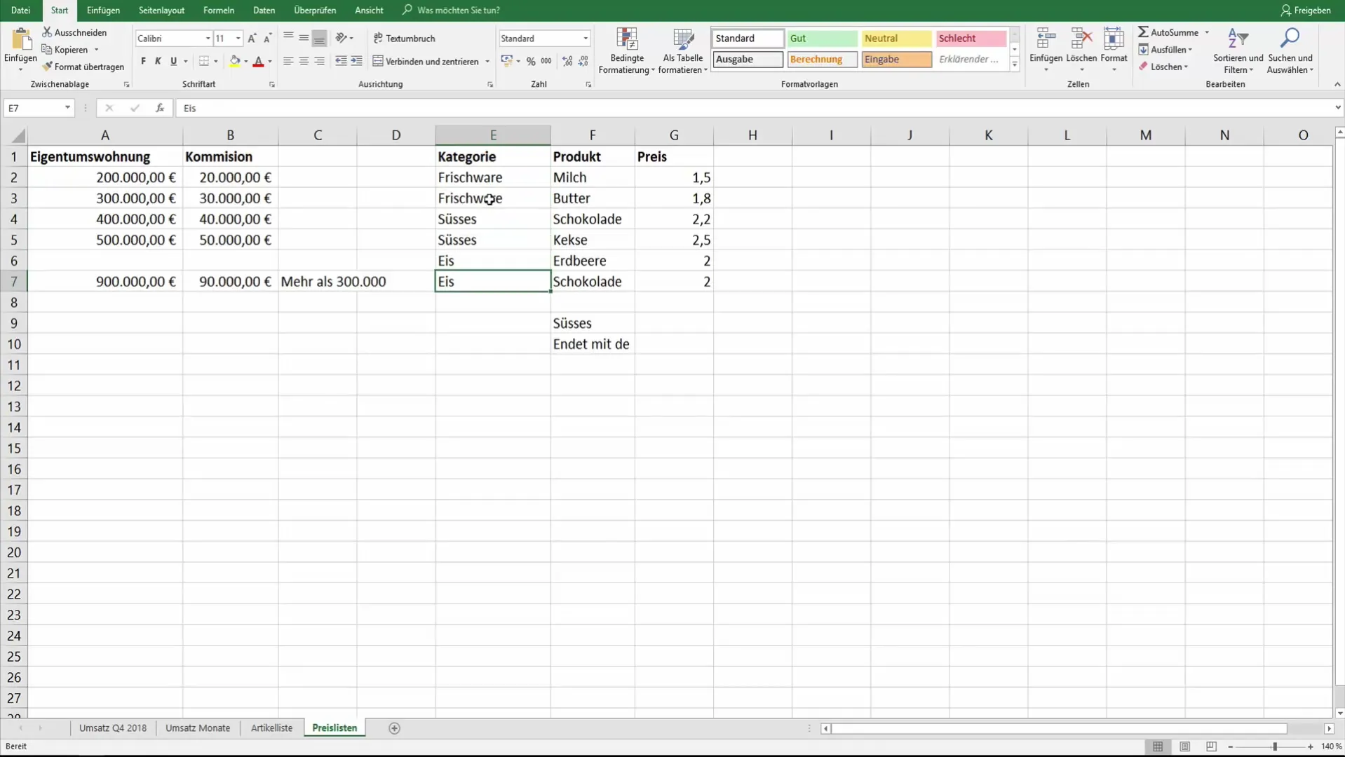
You create a list with various products and their prices. In the search range, you specify the category as "Sweets" to sum the prices of all sweet products, for example, €2.20 and €2.50.
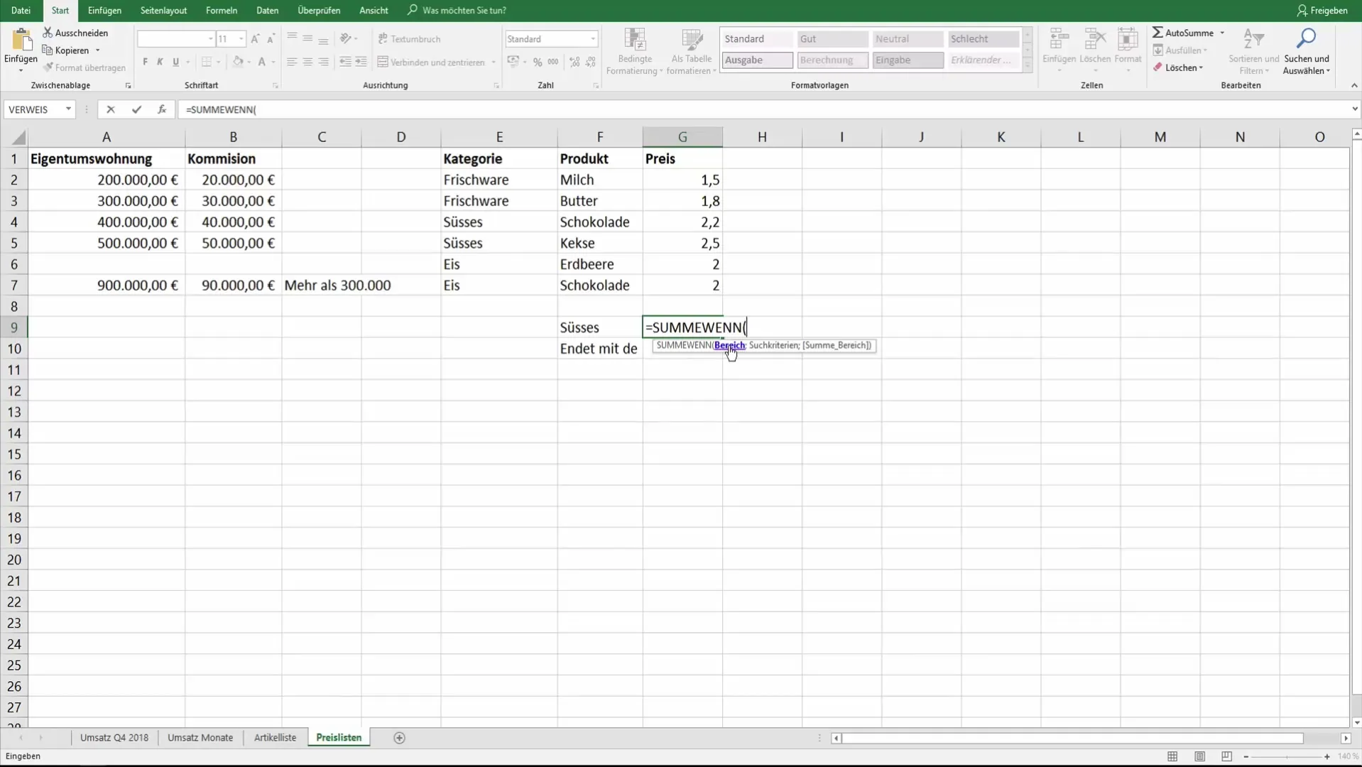
The function for this task is: =SUMIF(D2:D10, "Sweets", E2:E10), where D2:D10 is your search range for the categories, and E2:E10 is the price range.
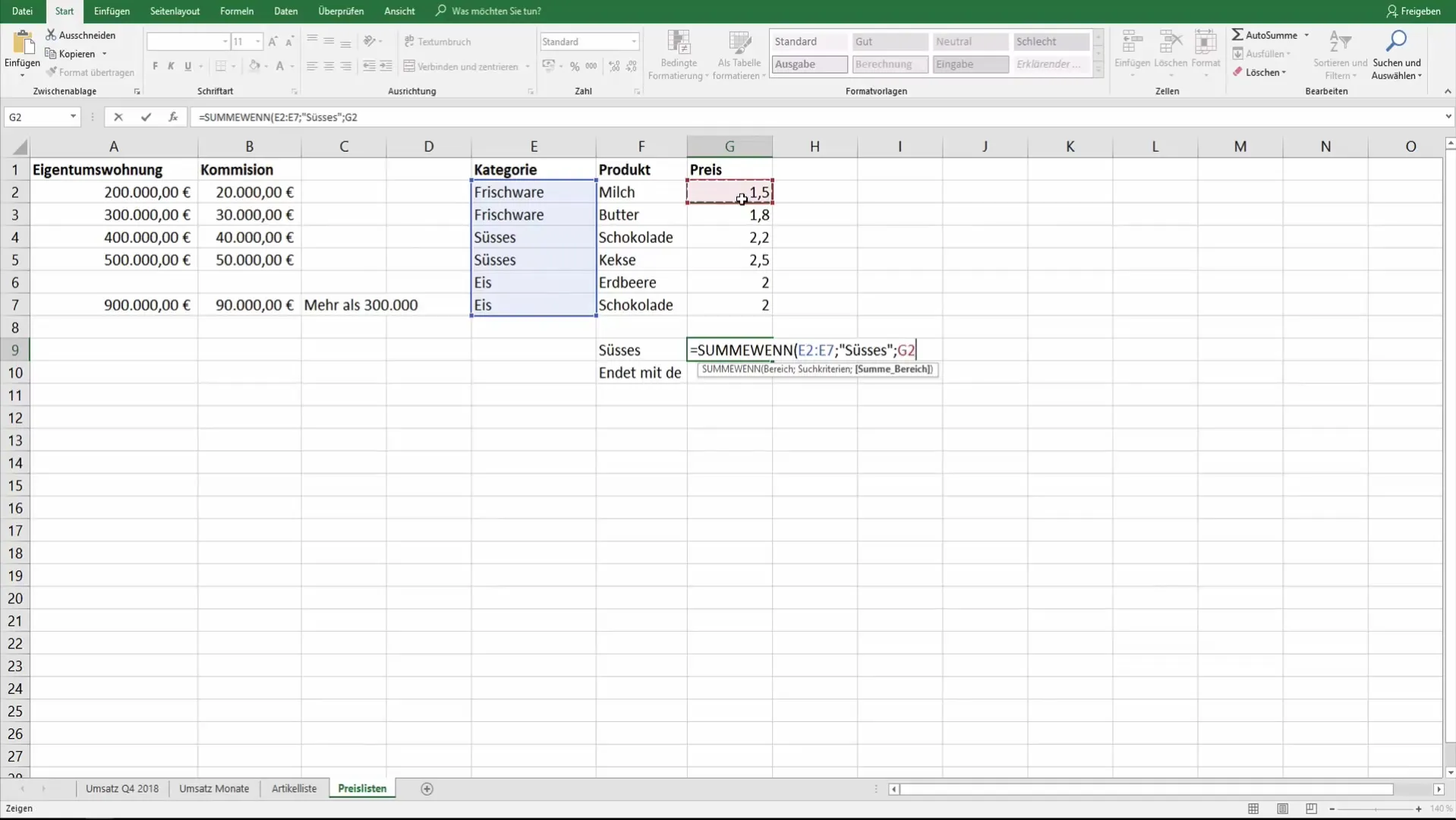
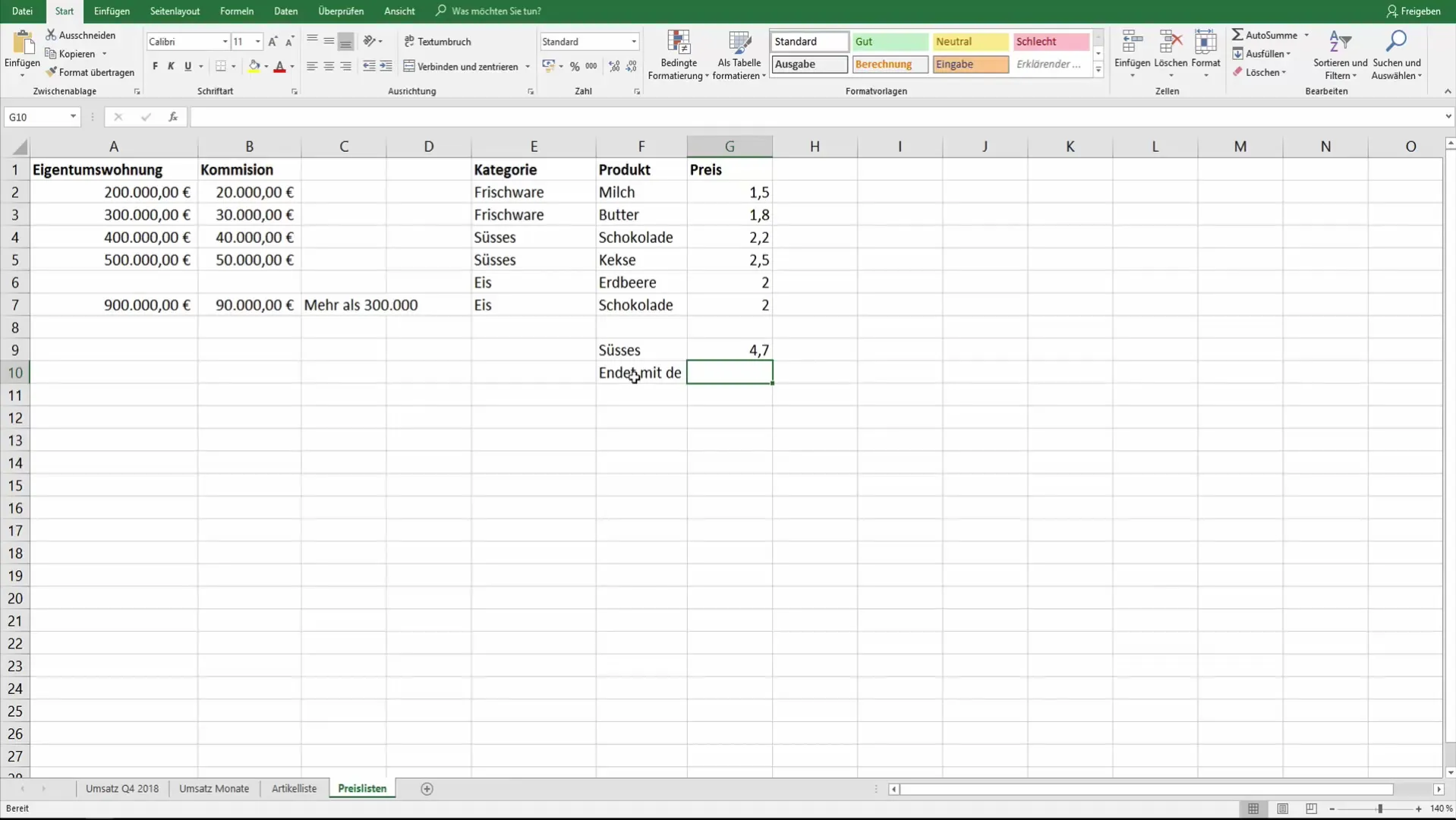
When you enter this formula, the total sum for the products in the "Sweets" category will be automatically calculated.
Using Wildcards
If you are searching for data that ends with specific letters (e.g., all products ending in "de"), you can use wildcards to refine the search.
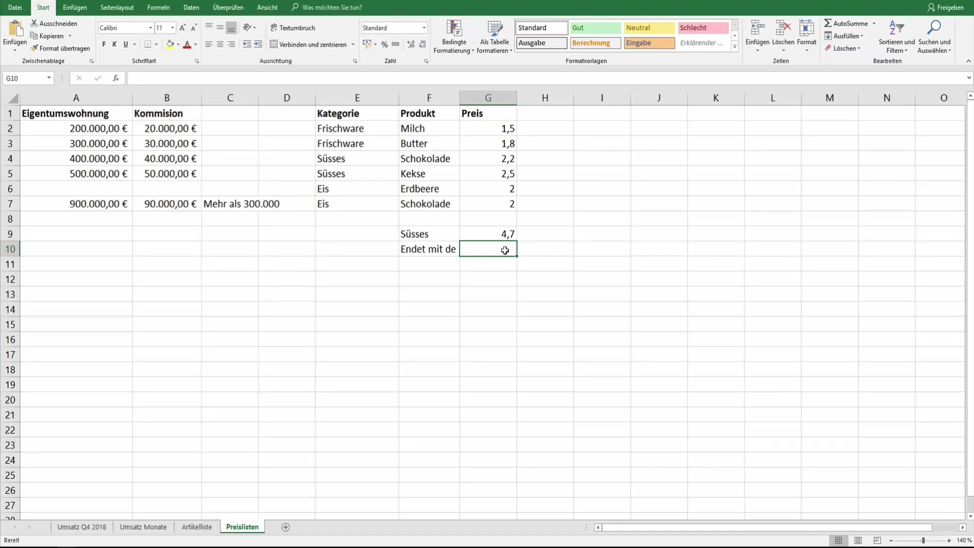
The formula could look like this: =SUMIF(D2:D10, "*de", E2:E10). Here, the asterisk (*) represents any characters that can precede "de."
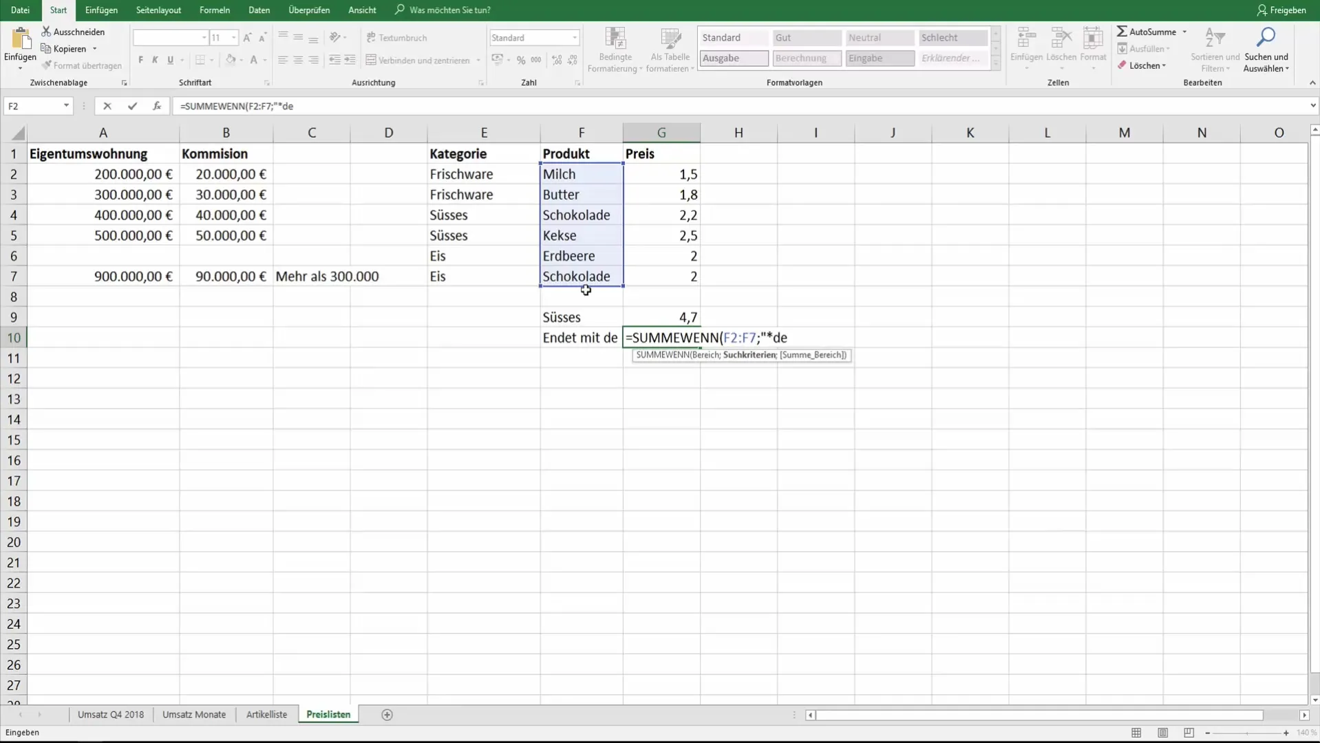
This flexible method allows you to capture multiple products that all end with "de" and calculate the corresponding total prices.

Conclusion and Practical Implementation
After working with the "SUMIF" function, you can combine different data and criteria to filter out specific information in your Excel data. Use the examples as a template and experiment with your own data.
Summary
By using the "SUMIF" function in Excel, you can easily and effectively sum specific values by applying simple criteria. Gain great advantages from the ability to also work with wildcards to refine your search.
Frequently Asked Questions
What is the "SUMIF" function?The "SUMIF" function sums values in a range based on a specific criteria.
How do I enclose criteria data in quotation marks?Criteria data such as ">300000" must be enclosed in quotation marks for Excel to correctly understand the queries.
Can I use wildcards with the "SUMIF" function?Yes, wildcards like the question mark (?) and asterisk (*) enable more flexible search criteria in the function.
What should I do if the search range does not match the sum range?The sum range must have the same number of rows or columns as the search range for the function to work correctly.
What should I do if I have additional questions?If you have further questions, please leave your inquiries in the comments below the video.
