Create a dynamic progress indicator in Excel

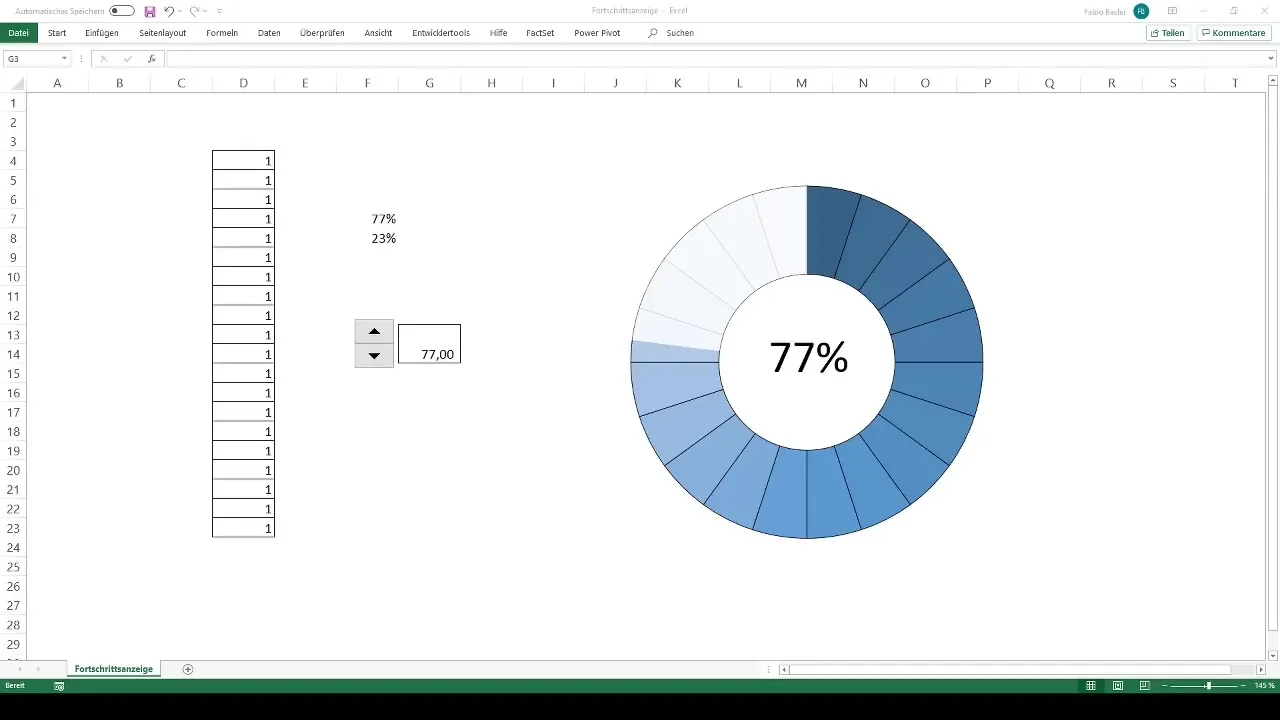
Excel is a powerful tool for data visualization, and one of the most impressive methods to present progress or goals is the dynamic progress indicator. In this guide, I will show you how to create an interactive doughnut chart that adjusts based on your input. You will learn how to achieve an appealing representation of your data using cell links and formulas.

Key Takeaways

• You can create a dynamic doughnut chart in Excel that reacts to input values.
• By linking cells and using formulas, the representation is adjusted in real time.
• Using drop-down lists and controls in Excel can increase user interactivity.

Step-by-Step Guide

Open a New Worksheet

Start by opening a new worksheet in Excel. You can do this by pressing the Alt and F11 keys simultaneously. Fresh data is crucial to build your progress indicator.

Prepare Data Input

For your progress indicator, you need data input. Define a total of 20 values that you want to use. The values should be structured in a way that you can easily capture and adjust them.

Create Doughnut Chart

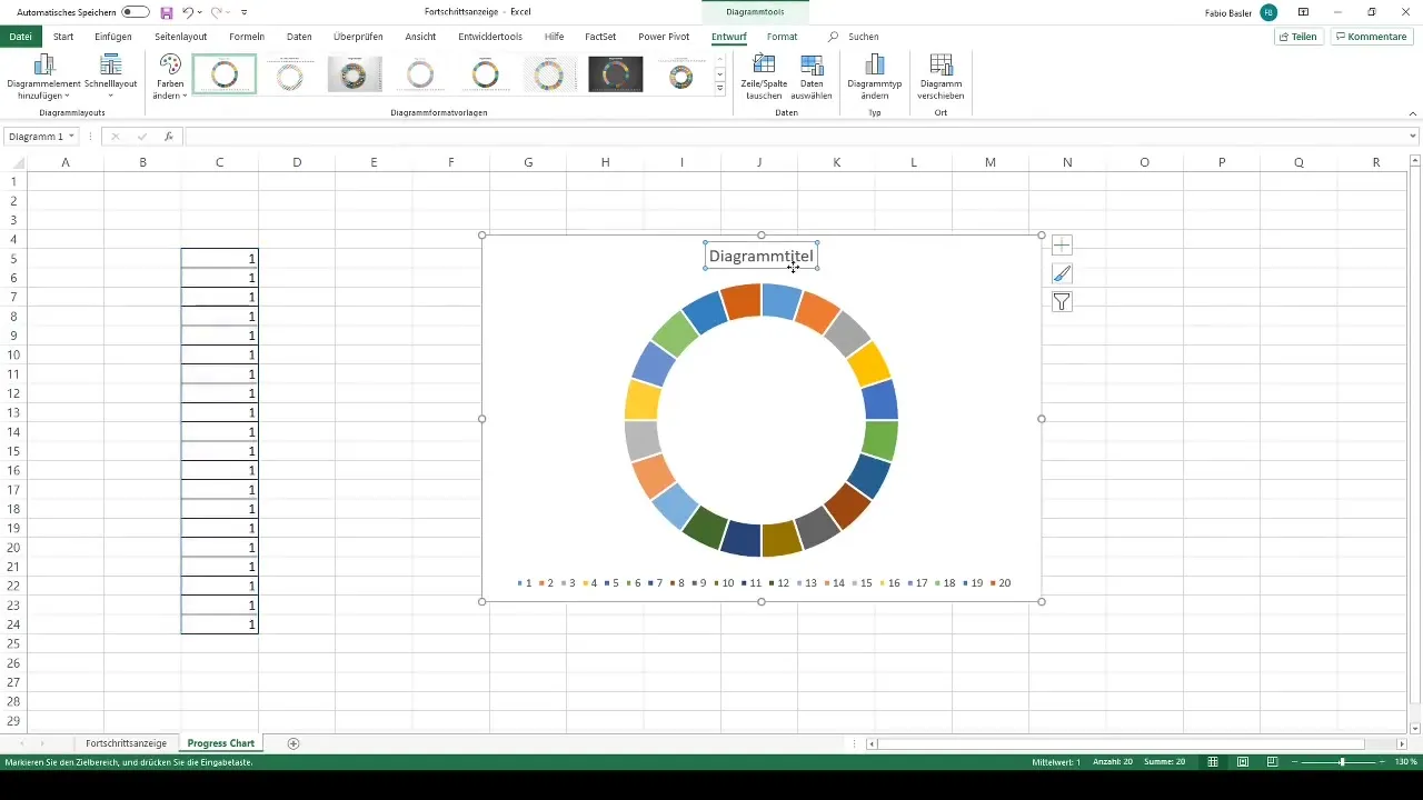
To create the doughnut chart, go to Insert and choose a simple doughnut chart. Remove the chart title and legend to make the representation clearer.

Format Chart

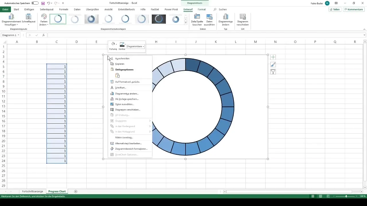
After creating the chart, you can customize the colors. Choose a blue tone for the chart and add a black outline to refine the design. Also remove the gridlines to further optimize the chart.

Add Second Doughnut Chart

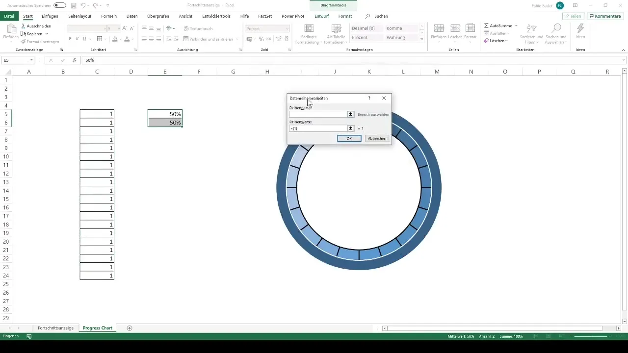
Add a second chart that follows the same format as the first one. Right-click on the chart and select Select Data to add a second data series. This allows you to integrate multiple rings in your display.

Combine Rings

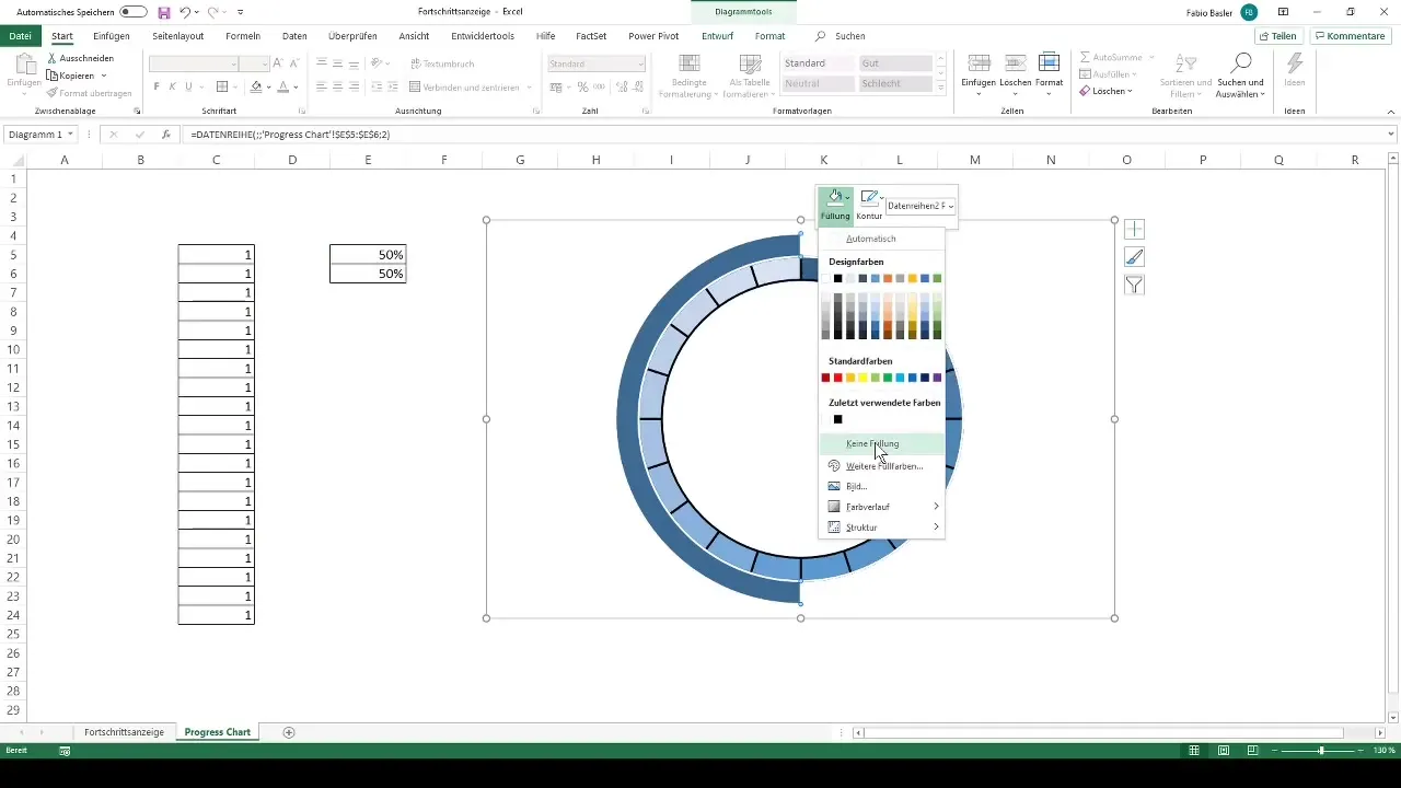
To make the representation clearer, you should combine the rings. This means placing one ring on top of the other. Click on the right semicircle of the chart, remove the fill, and adjust the transparency of the left ring.

Combine Chart Types

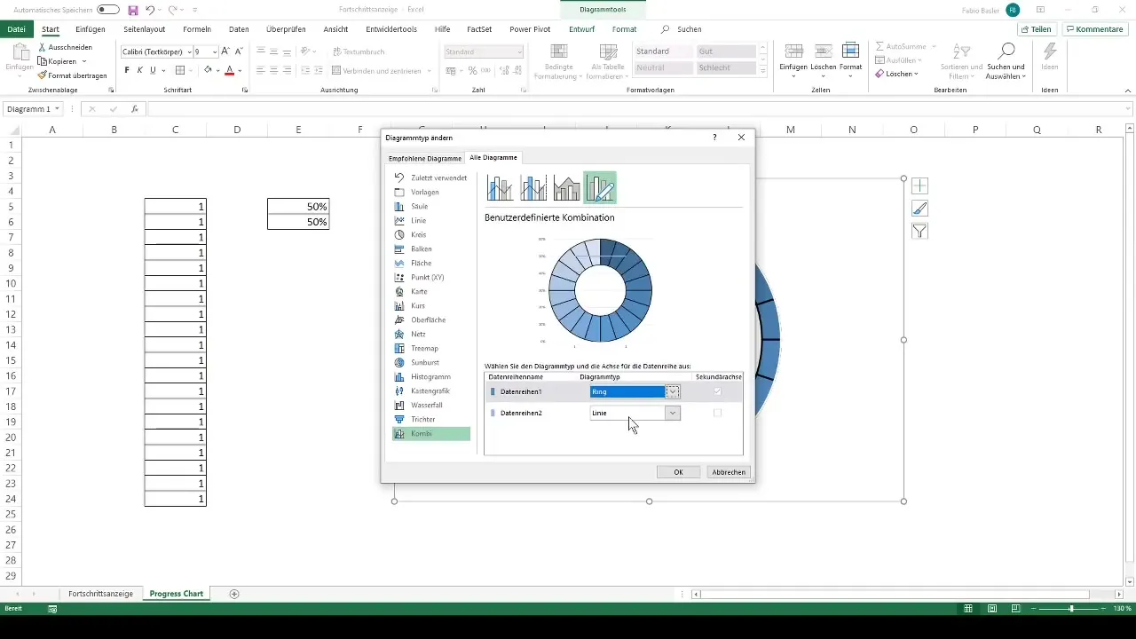
Change the chart type to a combo chart to combine two doughnut charts. Determine the secondary axis for the second data series and confirm the settings. This way, you will achieve the perfect visual representation of your values.

Formula to Calculate Counter Values

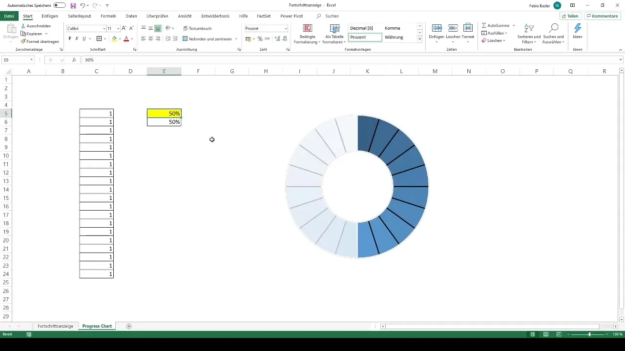
To ensure dynamic functionality, you need to create a formula that calculates the corresponding counter value. For example, if you input 50% into the chart, the chart should automatically adjust to display the value 50%.

Create Text Box for Percentage

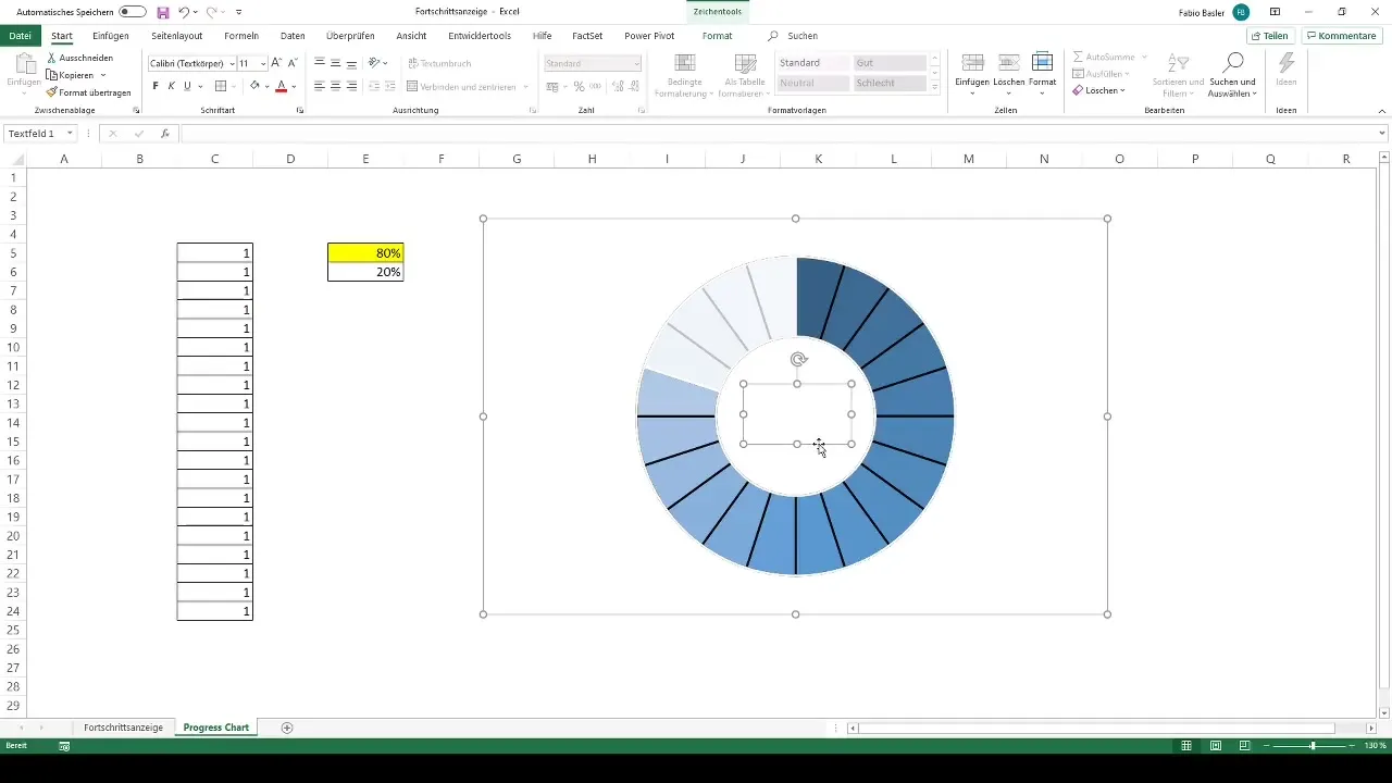
Add a text box inside the ring to display the current percentage. Link this text box to the cell containing the percentage value. This is done by entering an = symbol followed by the cell where your value is stored.

Add Interactive Drop-Down List

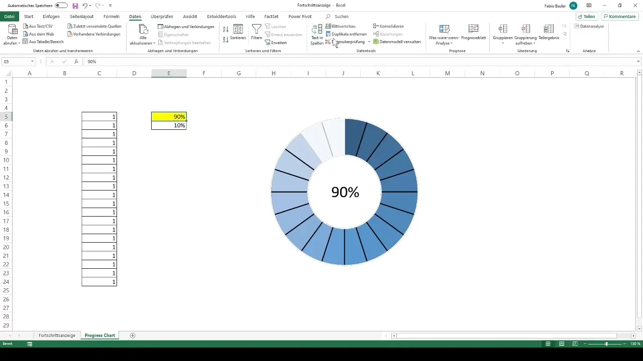
Create a dropdown list to adjust the percentage in steps. Go to Data and select Data Validation. Choose the option to create a list, and define the values you want to use (e.g. in 10% increments from 0 to 100%).

Enable User Interaction Controls

Activate Developer tools in Excel to use advanced functions. Add a spinner box whose values are linked to the data range of your choice. This allows you to quickly and easily adjust the value.

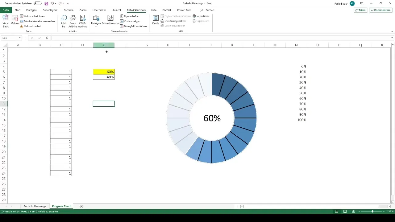
Linking Cells with the Spinner Box

Link the spinner box to the percentage by specifying the cell reflecting the current value. This allows you to experience the dynamics of the display in real time during use.

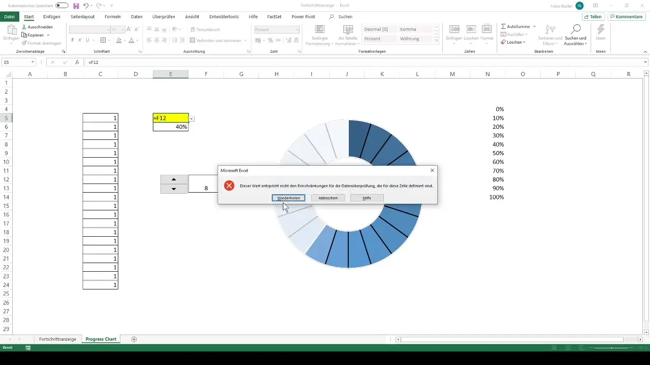
Display Customization

To ensure the display works correctly, you may need to adjust the formatting. Create a formula to display the values in percentages and make sure the display matches the current input.

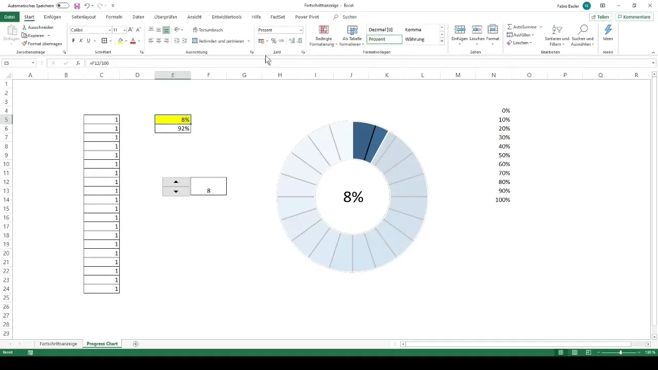
Summary

You have now learned how to create a dynamic progress indicator in Excel using pie charts, formulas, and interactive controls. This technique allows you to visualize progress in an engaging way and offers a great way to present data in an understandable format.