Set up traffic light function in Excel for data presentation

You want to make the data presentation in Excel more interesting? An traffic light function is an effective way to visually represent the status of values in a simple manner. With a clear visual representation, you can quickly determine whether your data is within the desired limits or not. In this guide, you will learn how to create a traffic light in Excel that changes to red, yellow, or green depending on the values entered.

Main takeaways:

• You will learn how to implement traffic light functions in Excel using conditional formatting.
• It explains how to use fonts to visually represent the traffic light.
• You will receive a step-by-step guide to set up and test the traffic light.

Step-by-Step Guide to Creating the Traffic Light Function

To create the traffic light in Excel, follow the steps below:

Step 1: Prepare Cells and Use the Webdings Font

First, open an Excel spreadsheet. Select cell D1 where you want to implement the traffic light function. To display the traffic light, use the font "Webdings." This font is available on every Windows system. Enter the letter "n" into cell D1.

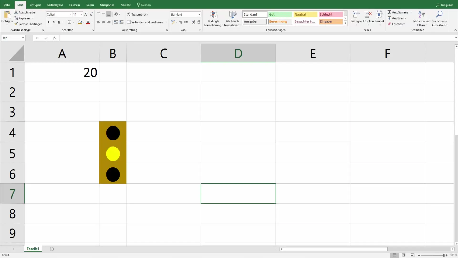
Copy cell D1 and paste it three times vertically so that you have three cells to represent the traffic light colors. Make sure to adjust the column width to make everything look good.

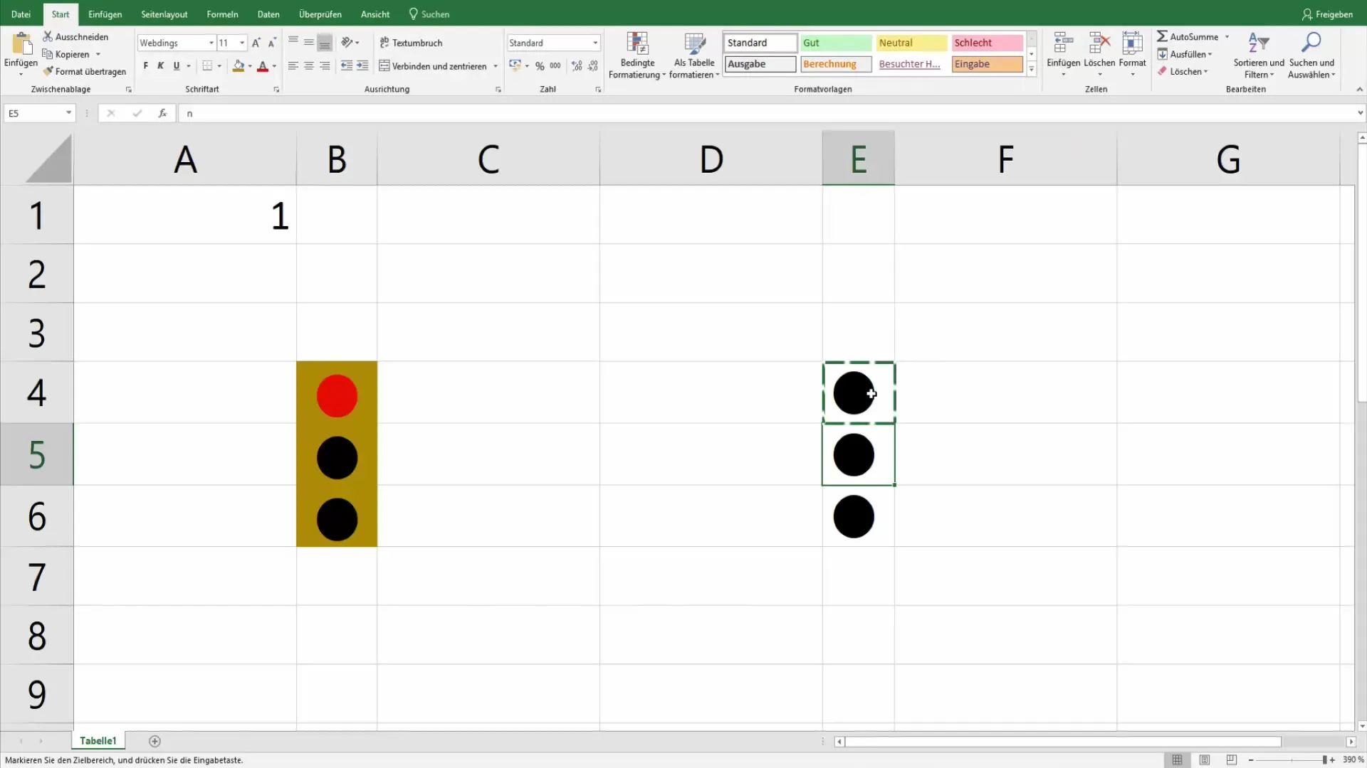
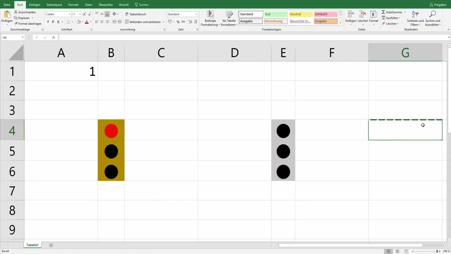
Align the cells horizontally and center the content. To achieve a clear distinction, design the background in a neutral color, such as a light gray.

Step 2: Set Conditional Formatting for Red

Now that your cells are created, it's time to set up conditional formatting for the traffic light colors. Start with the red light. Select cell D1 and go to the "Home" menu. Choose "Conditional Formatting" and then "New Rule".

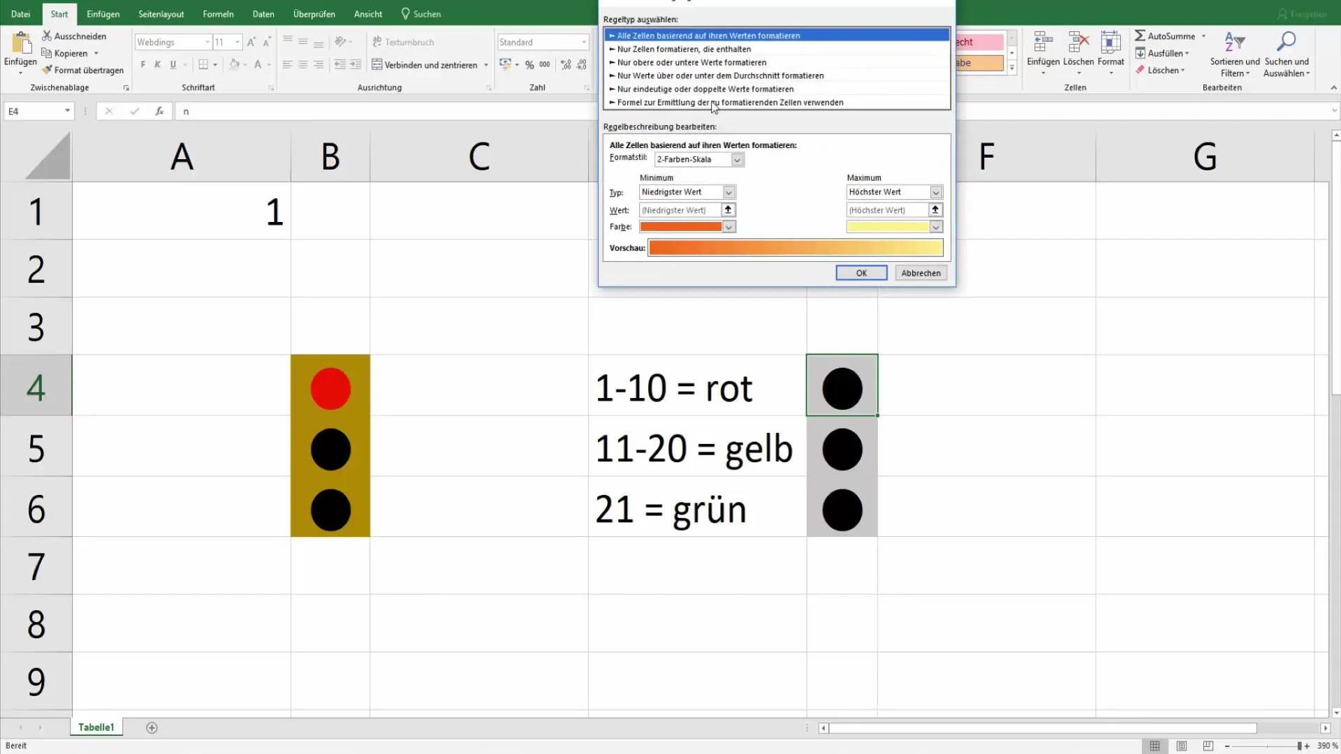
Select the option "Use a formula to determine which cells to format" and enter the following formula:

=D1<=10.

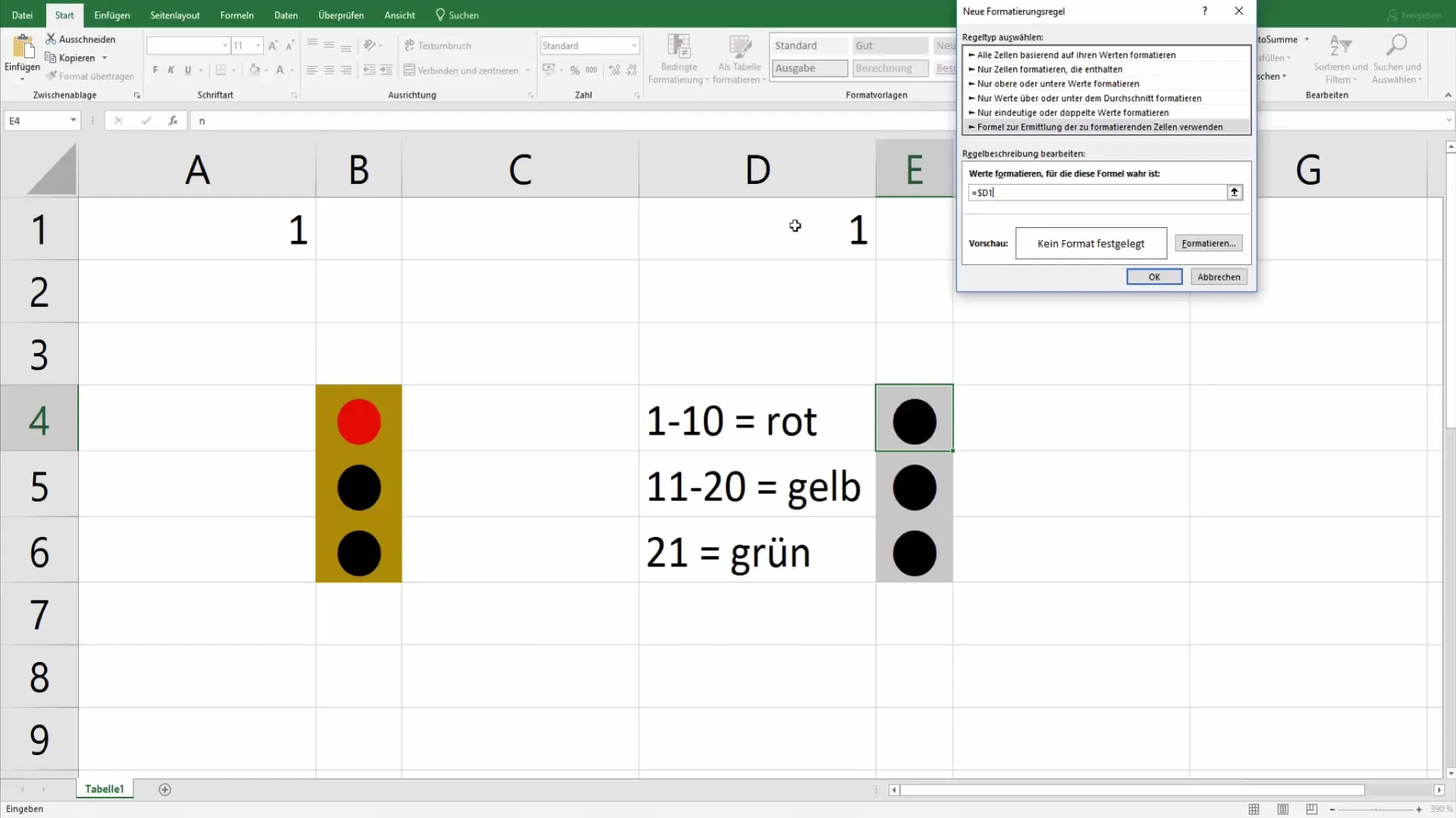
Click on "Format", select the font color red, and confirm with "OK". You will notice that the cell turns red when you enter a value equal to or less than 10.

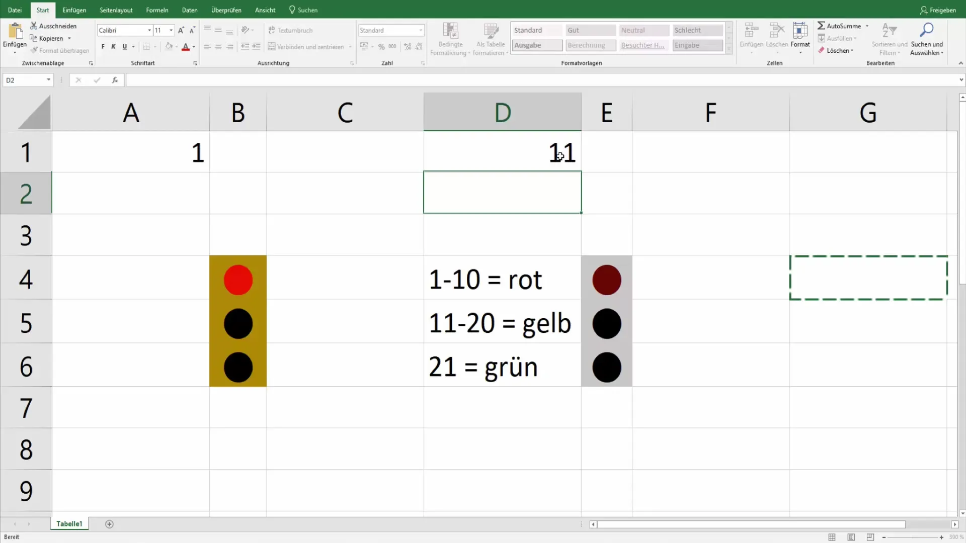
Step 3: Create Conditional Formatting for Yellow

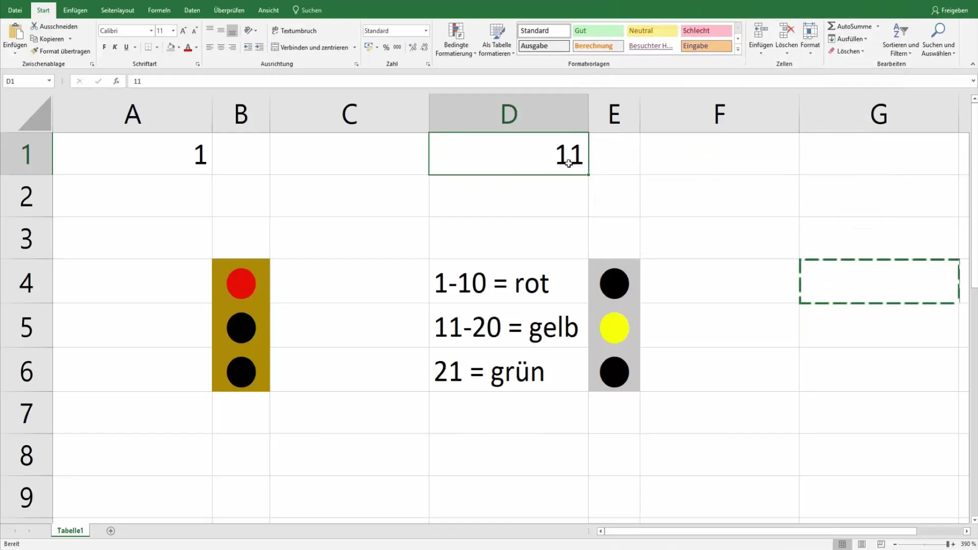
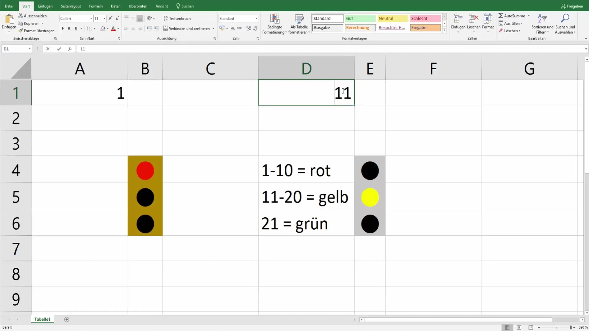
The next step is to set up the yellow light. Again, go to "Conditional Formatting" and create a new rule. Once again, use the option "Use a formula to determine which cells to format". In this case, enter the following formula to capture values between 11 and 20:

=AND(D1>10;D1<=20).

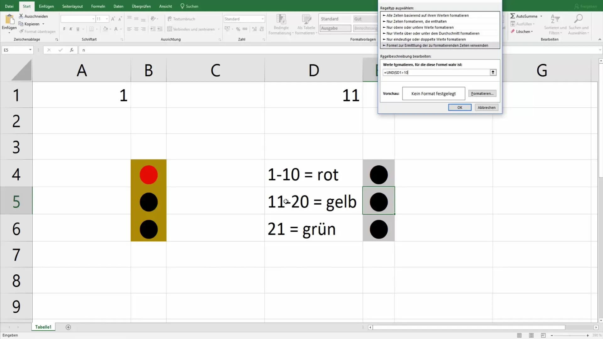
After entering the formula, click on "Format" again, select the color yellow. Confirm everything with "OK". Test the function by entering values in the corresponding range - the cell should now turn yellow when you enter a value between 11 and 20.

Step 4: Set Conditional Formatting for Green

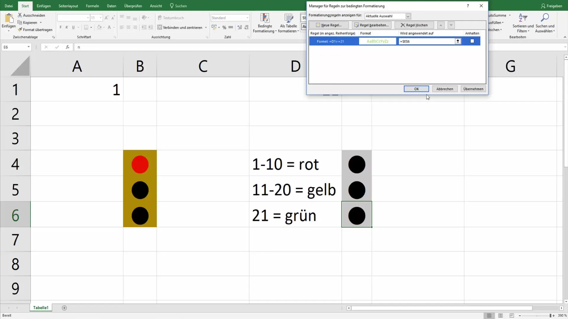
Now, set the final condition for the green light. Again, go to "Conditional Formatting" and add a new rule. Choose the formula "=D1>=21". This means the cell will turn green when the value is 21 or higher.

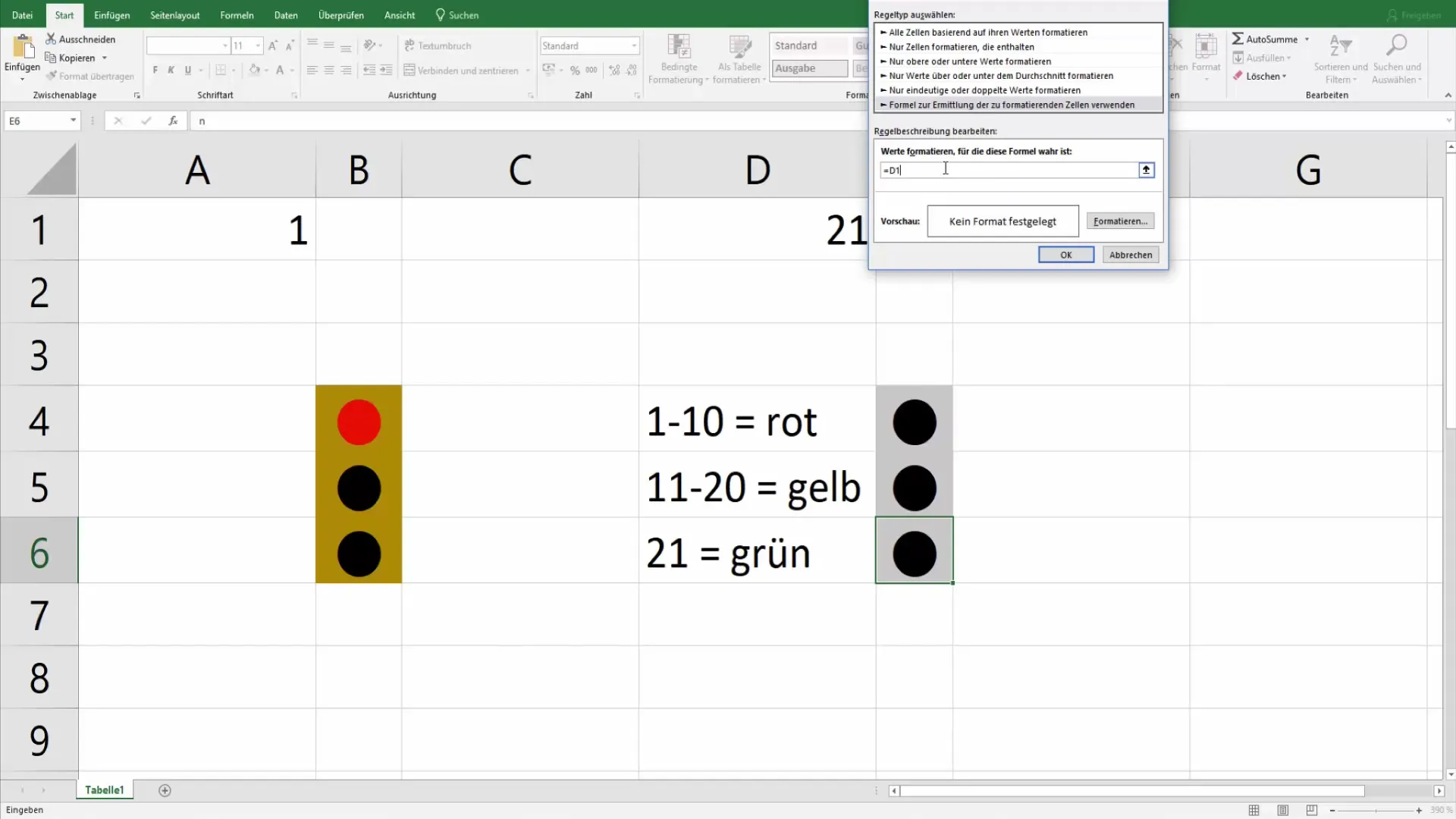
Choose the desired green font color as before and confirm your selection. Now the cell will turn green when you enter 21 or more, for example.

Step 5: Make further adjustments

To make further adjustments, you can also define conditions for empty cells. You can say that the cell will be displayed in red when the content is less than 1. Use conditional formatting again and add a rule for this.

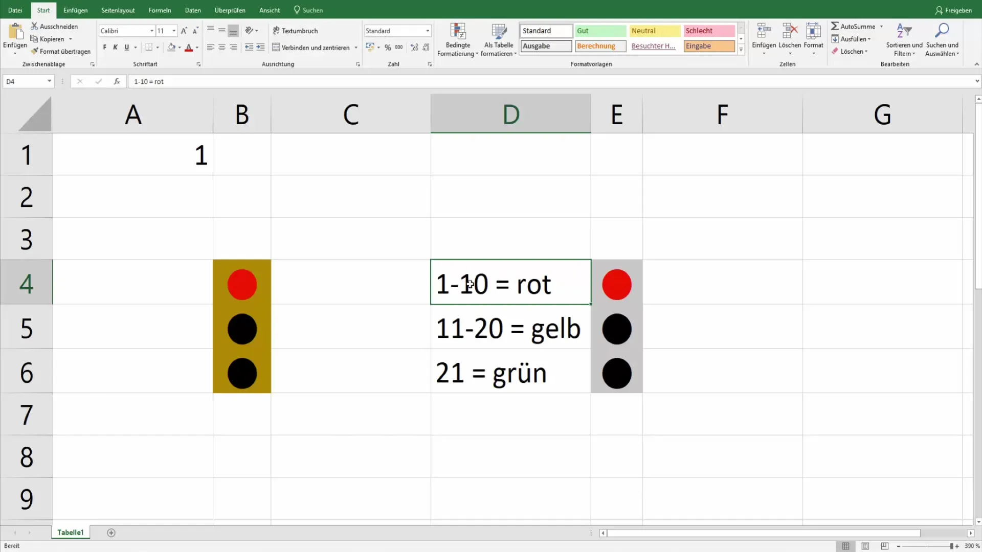
This rule gives you the ability to quickly recognize when, for example, the inventory level is zero or no relevant data has been entered.

Step 6: Test your traffic light

Now that all rules are defined, test the traffic light with different values. Enter values from 0 to 30 and observe how the colors change accordingly. This allows you to immediately understand the visual data presentation and act accordingly.

Summary

Through this simple step-by-step guide, you have learned how to set up a traffic light function in Excel that provides you with visual feedback on entered values. This can be extremely useful in many applications such as inventory levels, sales figures, or general KPI data.