Filter pivot tables in Excel

When working with pivot tables in Excel, you have an excellent opportunity to make your datasets more visually appealing. Pivot tables help you quickly analyze large amounts of data and gain important insights. A central aspect of this analysis is filtering. In this guide, you will learn how to effectively apply filters in pivot tables to retrieve specific information and optimize your data presentation.

Key Insights

• Filtering in pivot tables allows for targeted data analysis.
• You can apply and combine multiple filters simultaneously.
• Working with slicers can significantly simplify the filtering process.

Step-by-Step Guide

Applying Filters in Pivot Tables

To apply filters in your pivot table, start with the columns, rows, and values you have already set up. On the user interface, you will find filter options that allow you to search your datasets based on specific criteria.

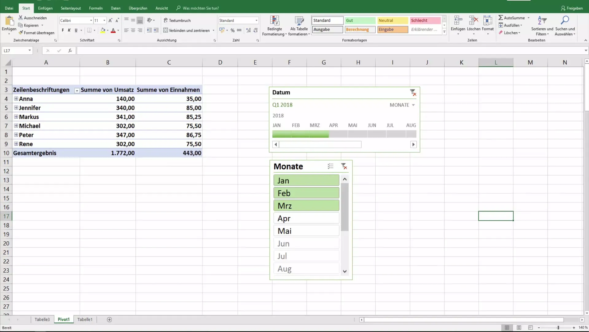
Filtering by Regions

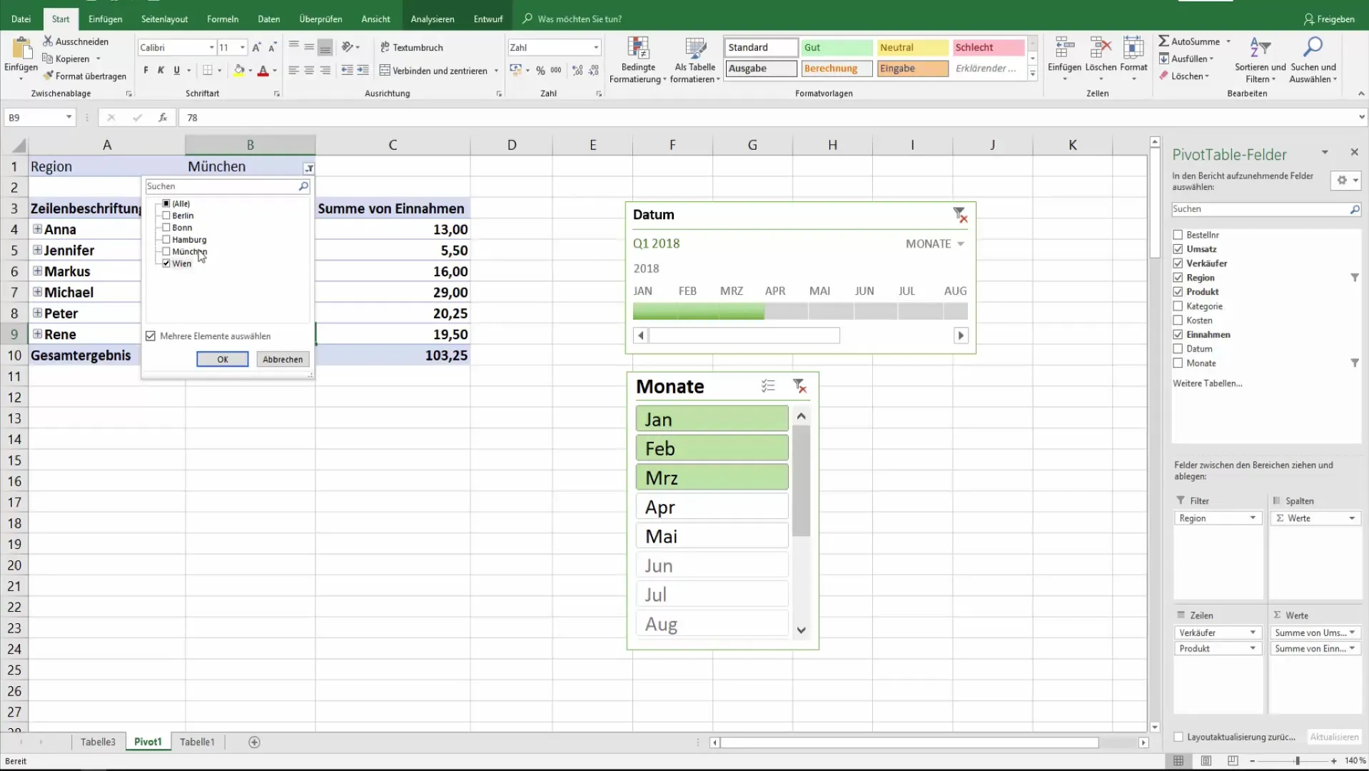
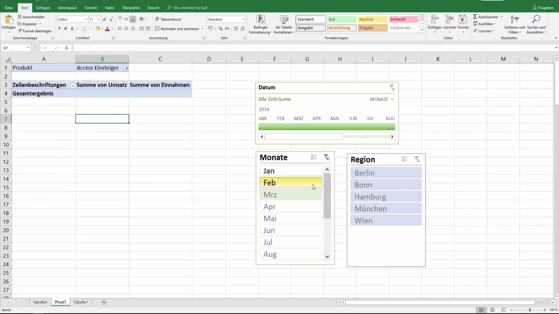
A common scenario is filtering by different regions. For example, you can filter sales based on regional criteria: Vienna, Munich, Bonn, or Berlin. To do this, simply click on the dropdown list next to the region and select the desired cities.

Multiple Selection of Filters

You have the option to apply multiple filters. To do this, hold down the control key (Ctrl) and click on the respective filter options you want to activate. This allows you to observe different cities simultaneously, such as sales from Vienna and Munich.

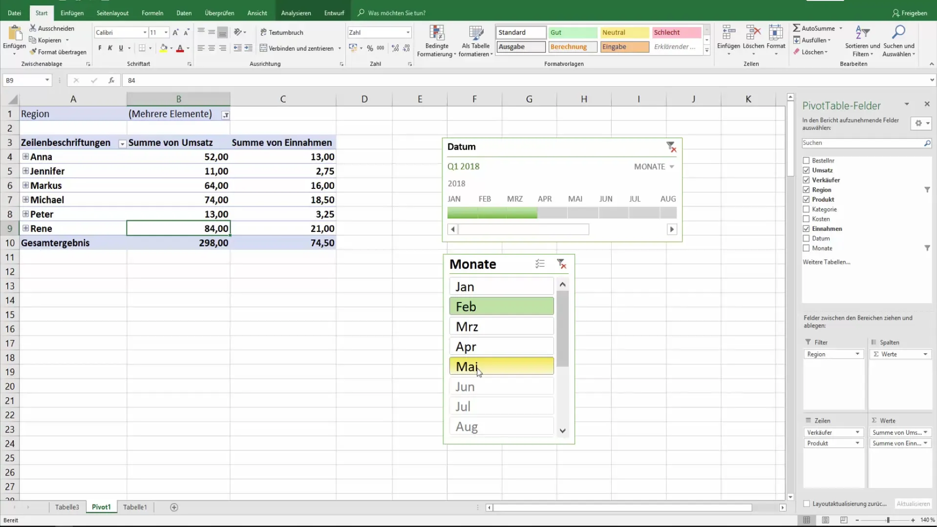
Combining Time and Region Filters

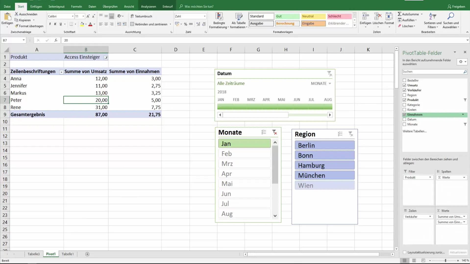
In addition to regional filters, you can also add temporal filters. For instance, if you want to analyze sales from January to May, you can set this time frame while simultaneously filtering by region. However, make sure not to have two overlapping active filters, as one will be set as inactive.

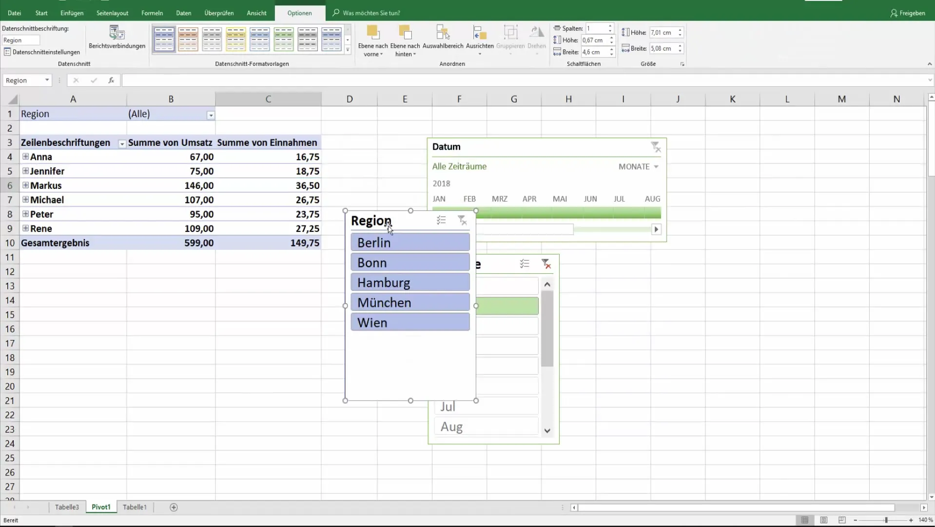
Using Slicers

A particularly useful function in Excel is the slicer. This allows for easy and visual selection of filters. You can insert it to, for example, choose the regions you are interested in. With a slicer, you can intuitively mark Berlin, Hamburg, Munich, or Vienna for sale without having to manually adjust the filter settings.

Filtering Products

Another approach to effective filtering is filtering by products. For example, do you have a specific product category you want to analyze? You can select products specifically, such as only "Exess Starter," to view their sales figures over the desired period.

Final Considerations

Filtering in pivot tables offers numerous ways to analyze your data precisely and effectively. Experiment with different filter combinations and utilize the tools Excel provides to deepen your data understanding. Remember that the ability to remove filters or ensure they are correctly ordered plays an important role in your data analysis.

Summary

You have learned how to use pivot tables in Excel to effectively filter your datasets. By applying multiple selections and using slicers, you have the tools to elevate your data analysis to the next level.