Create effective pivot tables in Excel

The use of pivot tables in Excel plays a crucial role in effective data analysis and presentation. Here you will learn how to create your own pivot tables in a few simple steps and how to use them optimally for your data analysis.

Key Takeaways

• Pivot tables help in analyzing and presenting large amounts of data in a clear manner.
• Correct preparation of your master and order data is essential.
• Pivot tables adjust dynamically as new data is added.
• Pivot charts allow for a graphical representation of pivot table data.

Step-by-Step Guide

Step 1: Establishing the Right Data Foundation

To create a pivot table, you need a complete data foundation. Ensure that all necessary column headings are present and that there are no blank rows or cells in your data. Segmenting your data into key columns like order number, revenue, seller, region, and products enhances the efficiency of your analyses.

Step 2: Converting Data into a Table

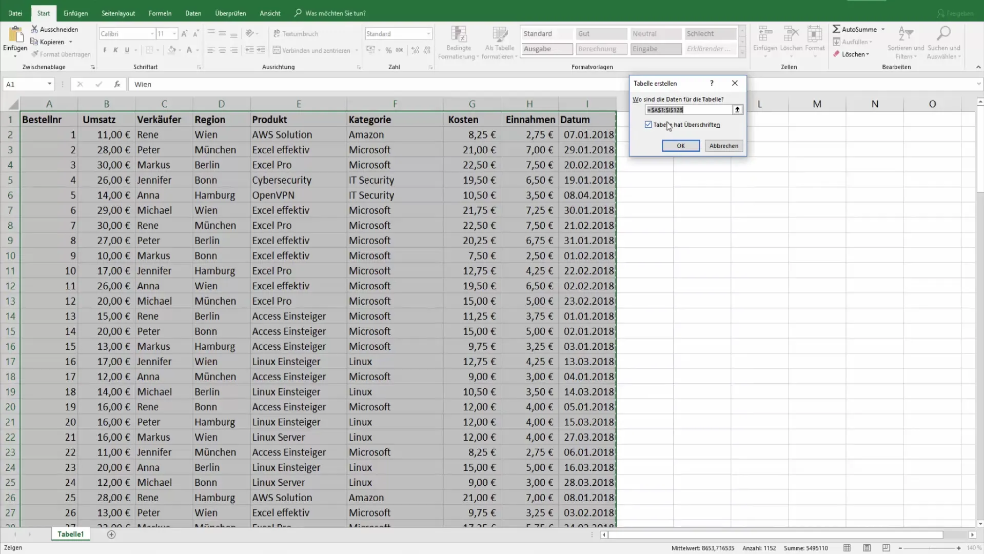
One of the best methods to keep your pivot table updated is by converting your data into an Excel table. Select your entire data range and press "Ctrl + T". This will automatically recognize the table, and you can assign it a name. This conversion facilitates easier editing and updating in the future.

Step 3: Creating the Pivot Table

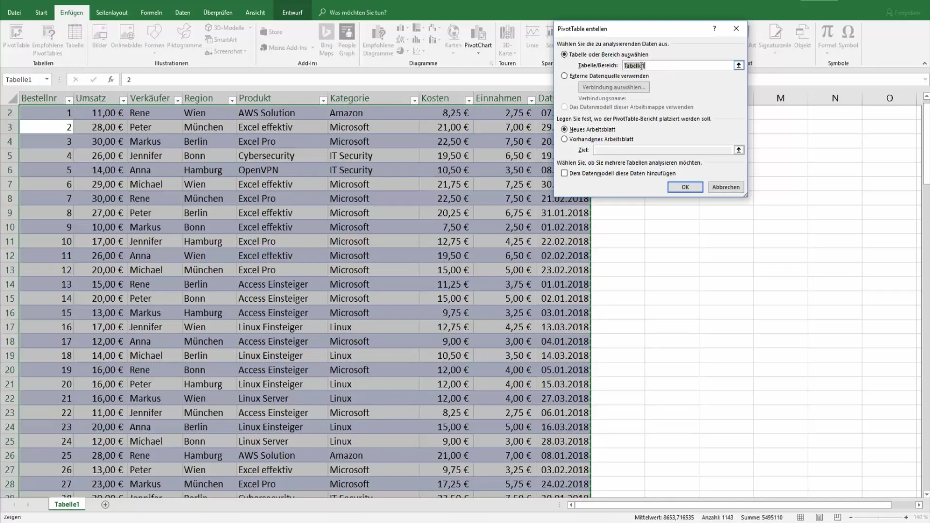
Now that you have converted your data into a table, you can begin creating the pivot table. Go to "Insert" and select "PivotTable". You can choose whether the pivot table should be placed in a new or existing worksheet. I recommend inserting it into a new worksheet for better clarity.

Step 4: Adjusting Pivot Fields

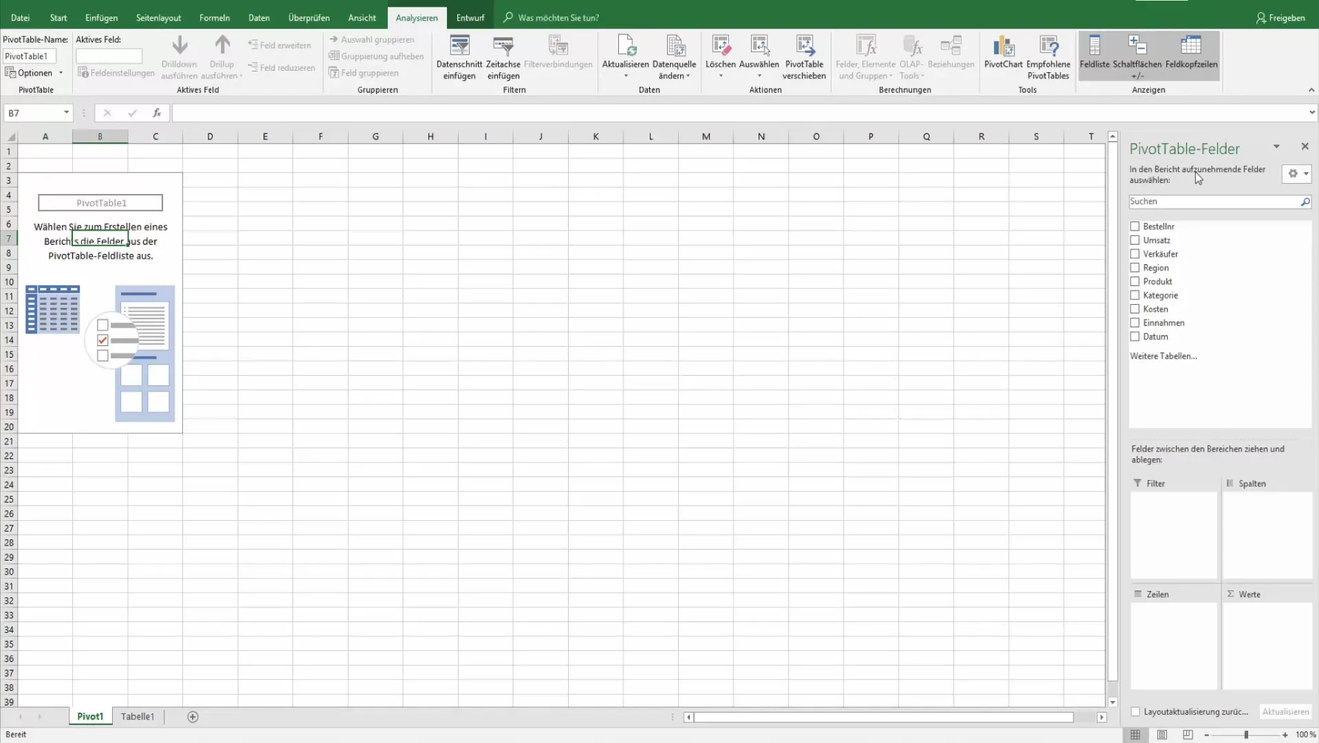
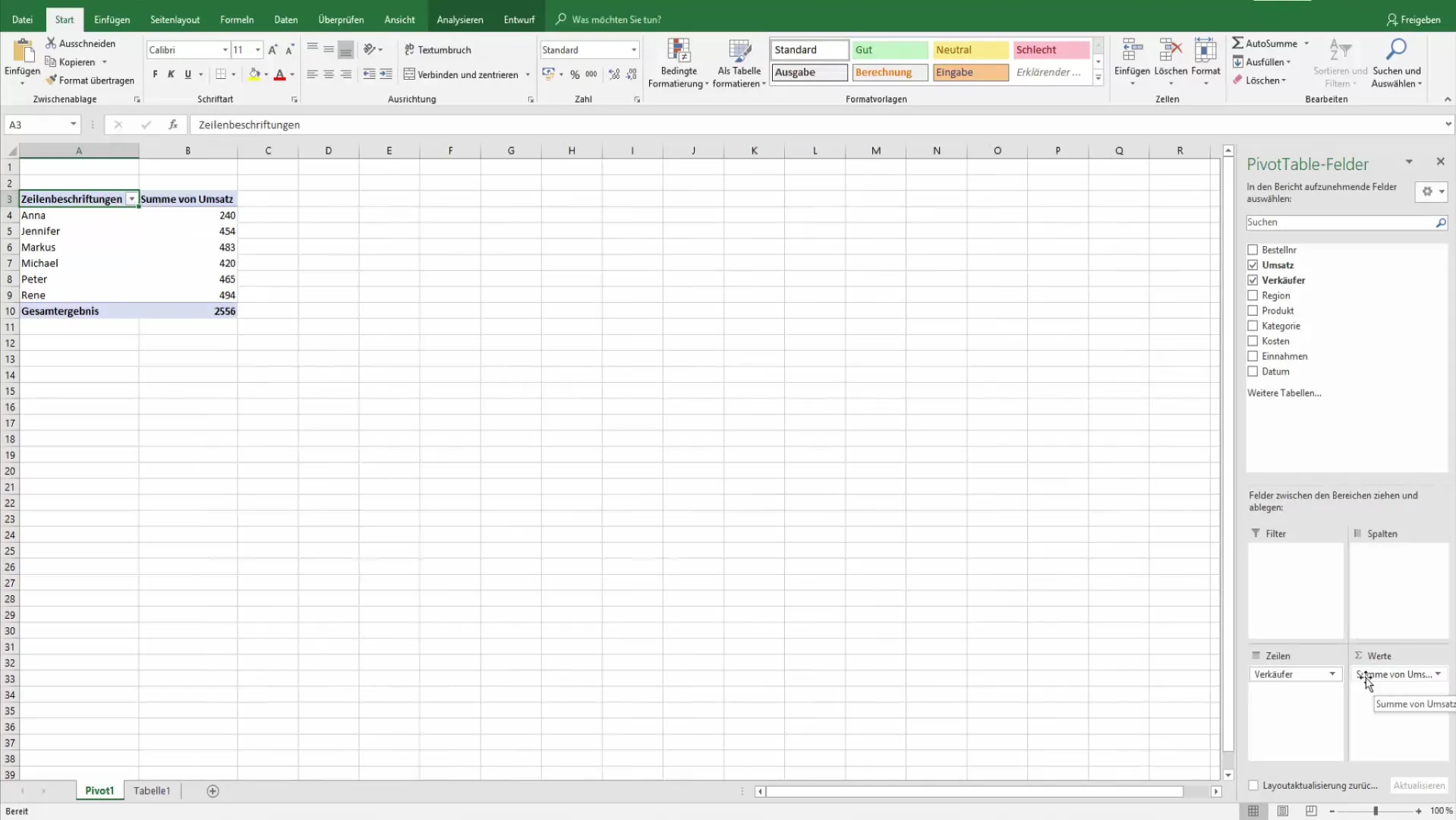
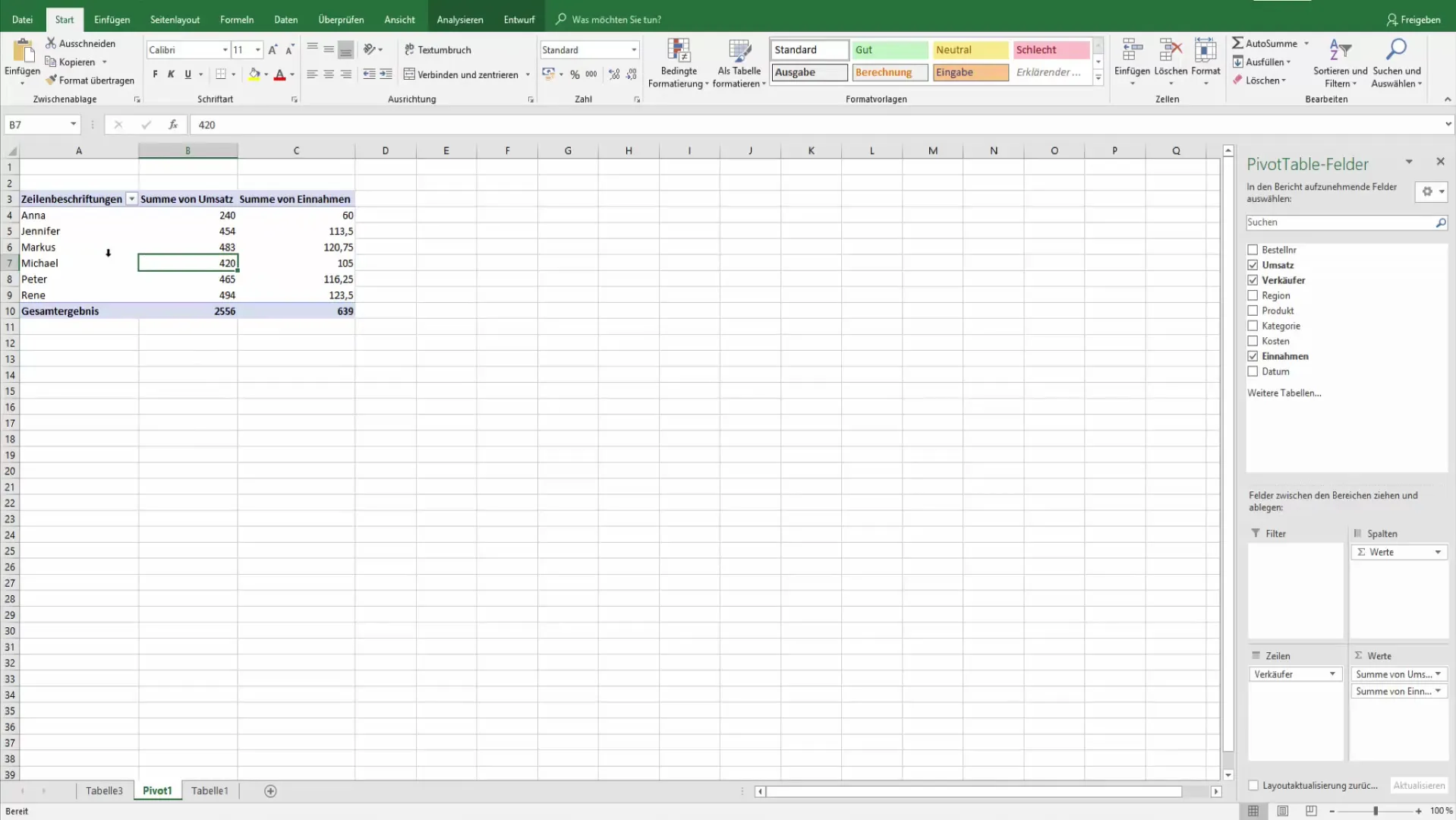
Once the pivot table is created, a field area will open on the right side of the screen where you can see the various fields of your table. Here, you can drag and drop fields to obtain the desired view of your data. For example, dragging "Seller" into the row area will list revenues by sellers.

Step 5: Adding Values and Analyzing

To display revenues in the pivot table, drag the revenue field into the values area. Excel will automatically sum revenues for each seller. You can always go back and adjust the fields to gain different insights into your data.

Step 6: Making Adjustments and Designing the Layout

After creating the pivot table, you can customize the layout to your preferences. Click on the "PivotTable Analyze" tab and here you can set various options for layout and design to enhance clarity. This includes adding filter options or changing formatting.

Step 7: Creating a Pivot Chart

If you want to visually represent your data, you can also create a pivot chart. Simply select the "PivotChart" option within your pivot table to obtain a visual representation of the analyzed data, making presentation significantly easier.

Step 8: Updating Data

If new data is added, you need to update the pivot table. Click on "PivotTable Analyze" and select "Refresh". This ensures that all new or modified information is incorporated into your analysis.

Summary

Using pivot tables provides a powerful method for evaluating and presenting large amounts of data. With the steps described, you can work efficiently and not only analyze your data but also present it understandably.