Working with data can be challenging, especially when it comes to identifying duplicate values. Often you receive a table from your supervisor and the task is to find duplicate entries. Fortunately, Excel offers an effective method to quickly and easily accomplish these tasks. In this tutorial, you will learn how to highlight duplicate values in Excel to save time and effort.
Key Takeaways
Conditional formatting in Excel is a powerful feature that allows you to quickly identify duplicate values. You can customize the formats to your liking, making it much easier to find duplicate entries. Furthermore, you can also analyze a single column instead of working directly with two columns.
Highlight Columns
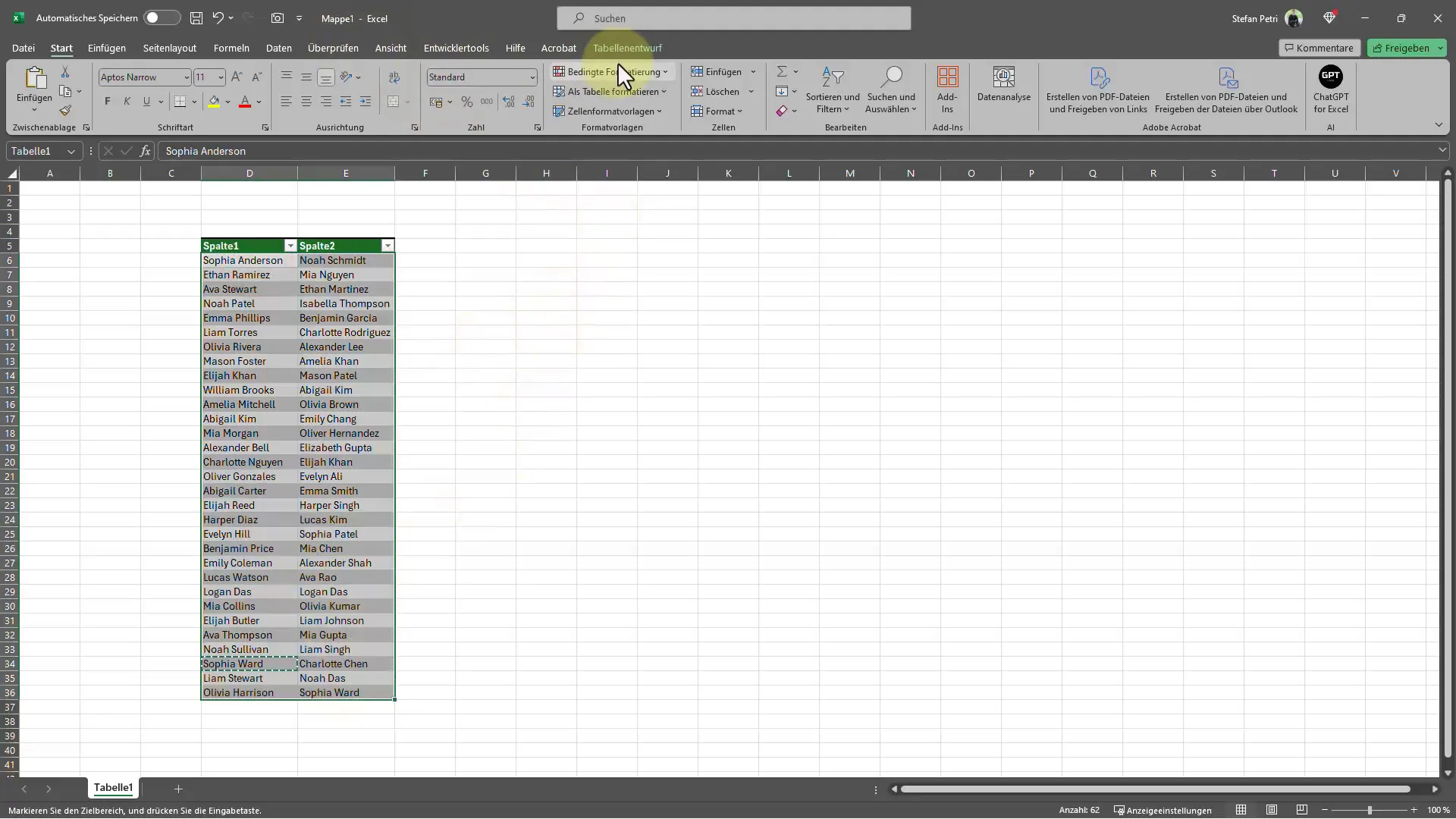
The first step is to highlight the columns you want to examine for duplicate values. Simply click on the first cell of the first column and drag the mouse pointer to the last row you want to analyze. Make sure you have both columns in your selection range.

Open Conditional Formatting
After highlighting the desired columns, switch to the "Home" tab in the top menu bar. There you will find the "Conditional Formatting," which is an important part of the process. Click on this button to open a dropdown menu.
Rule for Highlighting Cells
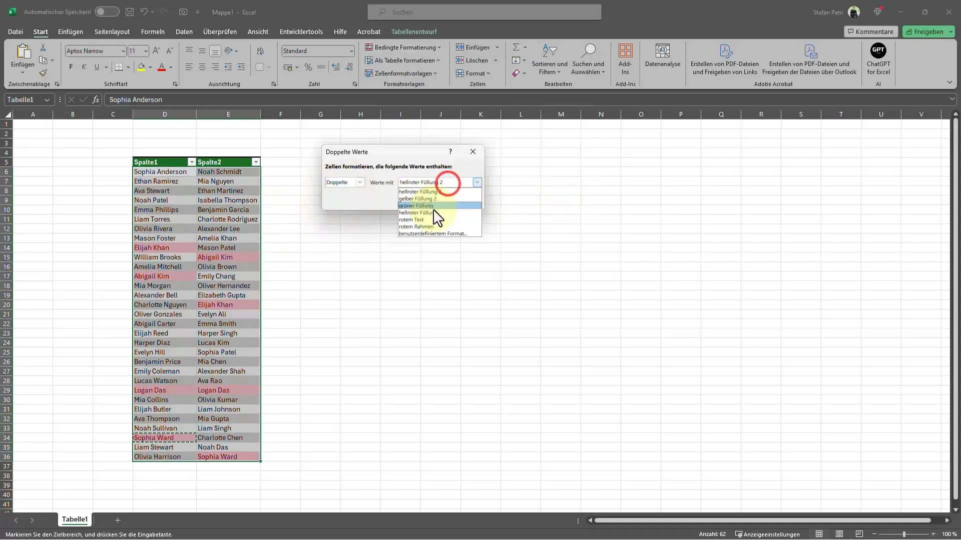
In the conditional formatting dropdown menu, you have the option to choose different rules. You want to select the "Highlight Cells' Rules" option. Then click on "Duplicate Values" to instruct Excel to search for duplicate entries in the selected columns.
Select Formatting
After choosing the rule, a new window will open where you can select the format for the highlighted values. You have the choice of different color tones, such as red for duplicate text or green for unique. Choose the color that is most intuitive and eye-catching for you, and click "OK".
Review the Results
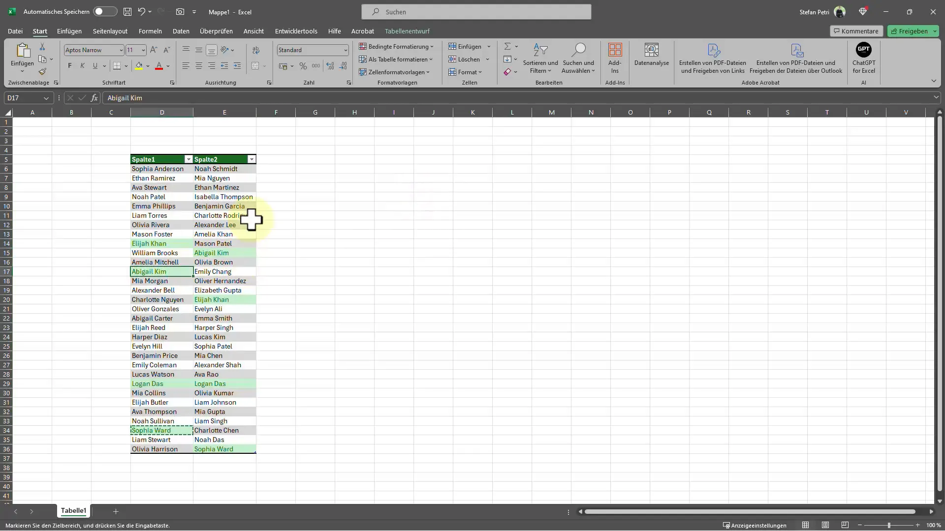
Now you have highlighted the duplicate values in your table with colors. Examine the table closely to determine which entries have duplicate content. This method is particularly handy as it gives you instant visual feedback and significantly speeds up the work.
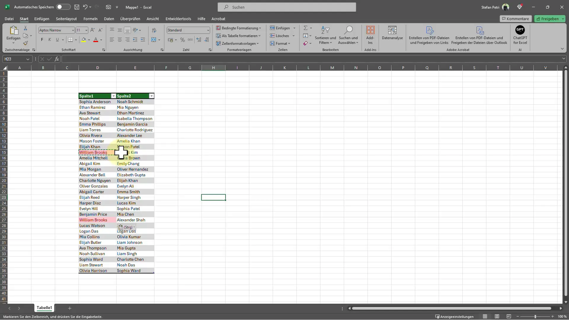
If you decide to only examine a single column for duplicate values, you can apply the same method. Just highlight the relevant column and follow the previous steps to create a rule for duplicate values. Excel will once again show you the duplicate entries.
To provide a specific example, imagine you have a list of names in one column. You copy a name and paste it in another row of the same column. When you apply conditional formatting, Excel will show you that this name is duplicated. You can then choose to highlight or delete this entry, depending on the necessity.
Summary - Excel Tips: Quickly Identify and Highlight Duplicate Values
In this guide, you have learned how to quickly and efficiently identify duplicate values in Excel. The main steps include highlighting the relevant columns, opening conditional formatting, selecting the rule for duplicate values, and setting a highlight format. By using this function, you can quickly identify and take action on unwanted duplicate entries.
Frequently Asked Questions
How do I find duplicate values in multiple columns?You need to highlight both columns, then use conditional formatting and choose the rule for duplicate values.
Can I customize the colors of the highlighted values?Yes, in the rule for duplicate values, you can choose the format according to your preferences.
Does the method also apply to a single column?Yes, you can apply the same method to a single column as well.
What should I do if I want to delete the duplicate values?After Excel highlights the duplicate entries, you can manually delete them.
What if I want to remove the formatting later?You can remove the conditional formatting by going to the "Conditional Formatting" menu and then "Manage Rules".


